Content from Getting Started
Last updated on 2024-05-01 | Edit this page
Overview
Questions
- How do I use JupyterLab?
- How can I run Python code in JupyterLab?
Objectives
- Learners are aware of applications for Python in library and information-science work environments.
- Learners can launch JupyterLab and create a Jupyter Notebook.
- Learners are able to navigate the JupyterLab interface.
- Learners are able to write and run Python cells in a notebook.
- Learners are able to save their code as an iPython notebook (.ipynb file).
Why Python?
Python is a popular programming language for tasks such as data collection, cleaning, and analysis. Python can help you to create reproducible workflows to accomplish repetitive tasks more efficiently.
This lesson works with a series of CSV files of circulation data from the Chicago Public Library system to demonstrate how to use Python to clean, analyze, and visualize usage data that spans over the course of multiple years.
Python in Libraries
There are a lot of ways that library and information science folks use Python in their work. Go around the room and have helpers and co-teachers share how they have used Python.
Learners: Can you think of other ways to use Python in libraries? Do you have hopes for how you’d like to use Python in the future?
Here a few areas where you might apply Python in your work.
Metadata work. Many cataloging teams use Python to migrate, transform and enrich metadata that they receive from different sources. For example, the pymarc library is a popular Python package for working with MARC21 records.
Collection and citation analysis. Python can automate workflows to analyze library collections. In cases where spreadsheets and OpenRefine are unable to support specific forms of analysis, Python is a more flexible and powerful tool.
Assessment. Library workers often need to collect metrics or statistics on some aspect of their work. Python can be a valuable tool to collect, clean, analyze, and visualize that data in a consistent way over time.
Accessing data. Researchers often use Python to collect data (including textual data) from websites and social media platforms. Academic librarians are often well-positioned to help teach these researchers how to use Python for web scraping or querying Application Programming Interfaces (APIs) to access the data they need.
Analyzing data. Python is widely used by scholars who are embarking on different forms of computational research (e.g., network analysis, natural language processing, machine learning). Library workers can leverage Python for their own research in these areas, but also take part in larger networks of academic support related to data science, computational social sciences, and/or digital humanities.
Use JupyterLab to edit and run Python code.
If you haven’t already done so, see the setup
instructions for details on how to install JupyterLab and Python via
Anaconda. The setup instructions also walk you through the steps you
should follow to create an lc-python folder on your
Desktop, and to download and unzip the dataset we’ll be working with
inside of that directory.
Getting started with JupyterLab
To run Python, we are going to use Jupyter Notebooks via JupyterLab. Jupyter notebooks are common tools for data science and visualization, and serve as a convenient environment for running Python code interactively where we can view and share the results of our Python code.
Alternatives to Juypter
There are other ways of editing, managing, and running Python code. Software developers often use an integrated development environment (IDE) like PyCharm, Spyder or Visual Studio Code (VS Code), to create and edit Python scripts. Others use text editors like Vim or Emacs to hand-code Python. After editing and saving Python scripts you can execute those programs within an IDE or directly on the command line.
Jupyter notebooks let us execute and view the results of our Python code immediately within the notebook. JupyterLab has several other handy features:
- You can easily type, edit, and copy and paste blocks of code.
- It allows you to annotate your code with links, different sized text, bullets, etc. to make it more accessible to you and your collaborators.
- It allows you to display figures next to the code to better explore your data and visualize the results of your analysis.
- Each notebook contains one or more cells that contain code, text, or images.
Start JupyterLab
Once you have created the lc-python directory on your
Desktop, you can start JupyterLab by opening a shell command line
interface or by using Anaconda Navigator.
Mac users - Command Line
- Press the cmd + spacebar keys and search for
Terminal. Click the result or press return. (You can also findTerminalin yourApplicationsfolder, underUtilities.) - After you have launched Terminal, change directories to the
lc-pythonfolder you created earlier and typejupyter lab:
Windows users - Command Line
To start the JupyterLab server you will need to access the Anaconda Prompt.
Press the Windows Logo Key and search for
Anaconda Prompt, click the result or press enter.Once you have launched the Anaconda Prompt, type the command:
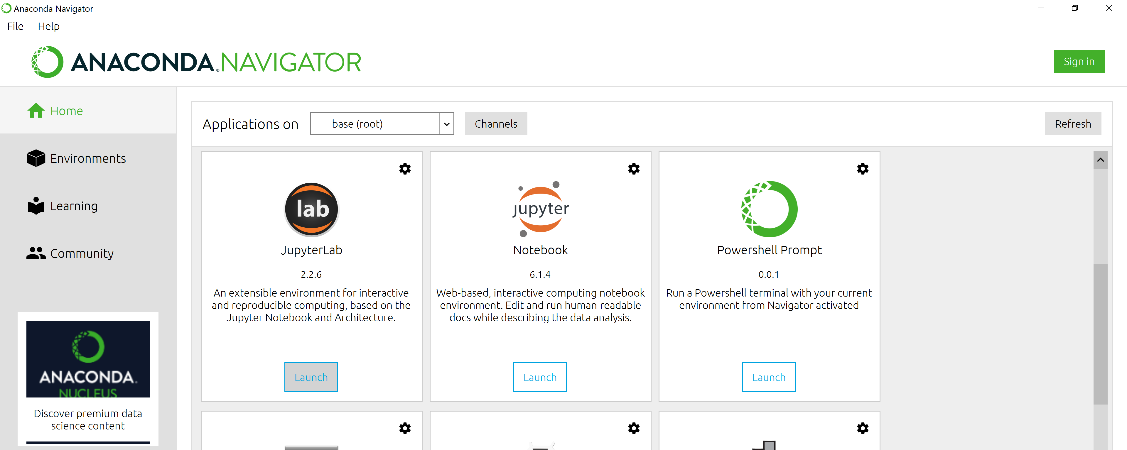
Start JupyterLab from Anaconda Navigator
If you are unfamiliar with the command line, you can launch
JupyterLab by opening the Anaconda Navigator app and choosing the
Launch button underneath the JuypterLab icon.
First start Anaconda Navigator (click for detailed instructions on macOS, Windows, and Linux). You can search for Anaconda Navigator via Spotlight on macOS (Command + spacebar), or by using the Windows search function (Windows Logo Key).
After you have launched Anaconda Navigator, click the
Launch button under JupyterLab. You may need to scroll down
to find it. Here is a screenshot of an Anaconda Navigator page similar
to the one that should open on either macOS or Windows.
The JupyterLab Interface
Launching JupyterLab opens a new tab or window in your preferred web
browser. While JupyterLab enables you to run code from your browser, it
does not require you to be online. If you take a look at the URL in your
browser address bar, you should see that the environment is located at
your localhost, meaning it is running from your computer:
http://localhost:8888/lab.
When you first open JupyterLab you will see two main panels. In the
left sidebar is your file browser. You should see a folder in the file
browser named data that contains all of our data.
Creating a Juypter Notebook
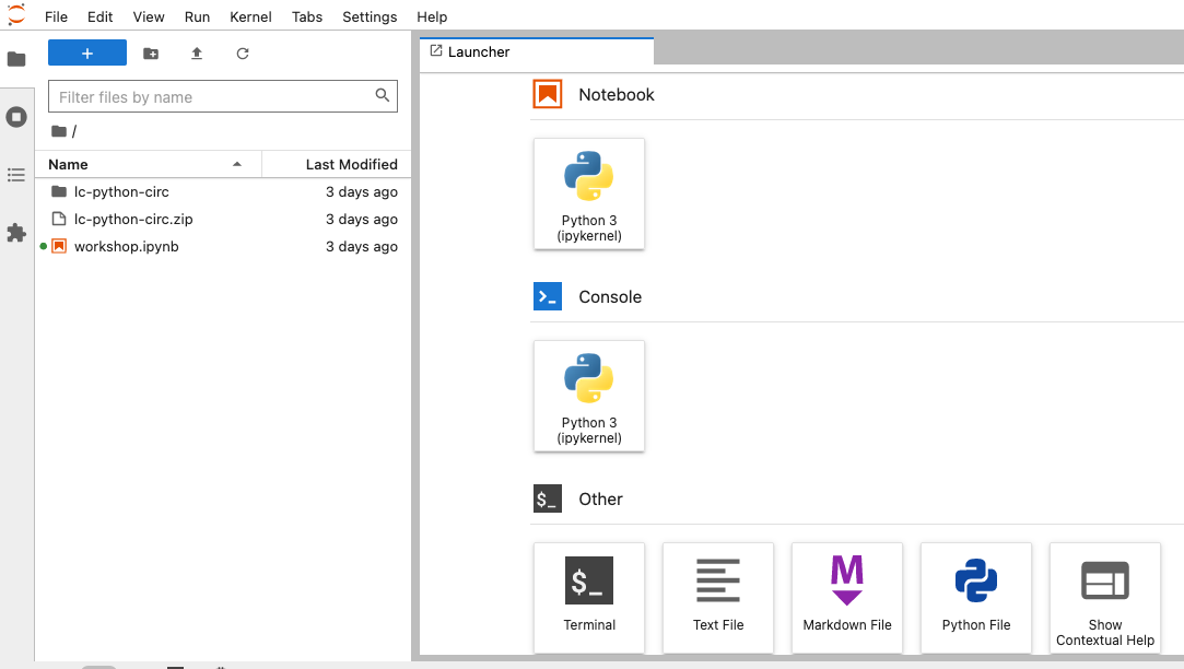
To the right you will see a Launcher tab. Here we have
options to launch a Python 3 notebook, a Terminal (where we can use
shell commands), text files, and other items. For now, we want to launch
a new Python 3 notebook, so click once on the
Python 3 (ipykernel) button underneath the Notebook header.
You can also create a new notebook by selecting New ->
Notebook from the File menu in the Menu Bar.
When you start a new Notebook you should see a new tab labeled
Untitled.ipynb. You will also see this file listed in the
file browser to the left. Right-click on the Untitled.ipynb
file in the file browser and choose Rename from the
dropdown options. Let’s call the notebook file,
workshop.ipynb.
JupyterLab? What about Jupyter notebooks? Python notebooks? IPython?
JupyterLab is the next stage in the evolution of the Jupyter Notebook. If you have prior experience working with Jupyter notebooks, then you will have a good idea of how to work with JupyterLab. Jupyter was created as a spinoff of IPython in 2014, and includes interactive computing support for languages other than just Python, including R and Julia. While you’ll still see some references to Python and IPython notebooks, IPython notebooks are officially deprecated in favor of Jupyter notebooks.
We will share more features of the JupyterLab environment as we advance through the lesson, but for now let’s turn to how to run Python code.
Running Python code
Jupyter allows you to add code and formatted text in different types of blocks called cells. By default, each new cell in a Jupyter Notebook will be a “code cell” that allows you to input and run Python code. Let’s start by having Python do some arithmetic for us.
In the first cell type 7 * 3, and then press the
Shift+Return keys together to execute the contents
of the cell. (You can also run a cell by making sure your cursor is in
the cell and choosing Run > Run Selected Cells or
selecting the “Play” icon (the sideways triangle) at the top of the
noteboook.)
You should see the output appear immediately below the cell, and Jupyter will also create a new code cell for you.
If you move your cursor back to the first cell, just after the
7 * 3 code, and hit the Return key (without
shift), you should see a new line in the cell where you can add more
Python code. Let’s add another calculation to the same cell:
While Python runs both calculations Juypter will only display the output from the last line of code in a specific cell, unless you tell it to do otherwise.
Editing the notebook
You can use the icons at the top of your notebook to edit the cells in your Notebook:
- The
+icon adds a new cell below the selected cell. - The scissors icon will delete the current cell.
You can move cells around in your notebook by hovering over the left-hand margin of a cell until your cursor changes into a four-pointed arrow, and then dragging and dropping the cell where you want it.
Markdown
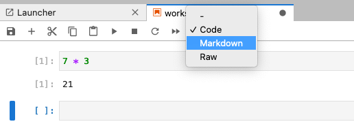
You can add text to a Juypter notebook by selecting a cell, and
changing the dropdown above the notebook from Code to
Markdown. Markdown is a lightweight language for formatting
text. This feature allows you to annotate your code, add headers, and
write documentation to help explain the code. While we won’t cover
Markdown in this lesson, there are many helpful online guides out there:
- Markdown
for Jupyter Cheatsheet (IBM) - Markdown Guide (Matt Cone)
You can also use “hotkeys”” to change Jupyter cells from Code to Markdown and back:
- Click on the code cell that you want to convert to a Markdown cell.
- Press the Esc key to enter command mode.
- Press the M key to convert the cell to Markdown.
- Press the y key to convert the cell back to Code.
Content from Variables and Types
Last updated on 2024-04-15 | Edit this page
Overview
Questions
- How can I store data in Python?
- What are some types of data that I can work with in Python?
Objectives
- Write Python to assign values to variables.
- Print outputs to a Jupyter notebook.
- Use indexing to manipulate string elements.
- View and convert the data types of Python objects.
Use variables to store values.
Variables are names given to certain values. In Python the
= symbol assigns a value to a variable. Here, Python
assigns the number 42 to the variable age and
the name Ahmed in single quote to a variable
name.
Use print() to display values.
You can print Python objects to the Jupyter notebook output using the
built-in function, print(). Inside of the parentheses we
can add the objects that we want print, which are known as the
print() function’s arguments.
OUTPUT
Ahmed 42 In Jupyter notebooks, you can leave out the print()
function for objects – such as variables – that are on the last line of
a cell. If the final line of Jupyter cell includes the name of a
variable, its value will display in the notebook when you run the
cell.
OUTPUT
42Format output with f-strings
F-strings provide a concise and readable way to format strings by
embedding Python expressions within them. You can format variables as
text strings in your output using an f-string. To do so, start a string
with f before the open single (or double) quote. Then add
any replacement fields, such as variable names, between curly braces
{}. (Note the f string syntax can only be used with Python
3.6 or higher.)
OUTPUT
'Ahmed is 42 years old'Variables must be created before they are used.
If a variable doesn’t exist yet, or if the name has been misspelled,
Python reports an error called a NameError.
ERROR
---------------------------------------------------------------------------
NameError                                 Traceback (most recent call last)
<ipython-input-1-c1fbb4e96102> in <module>()
----> 1 print(eye_color)

NameError: name 'eye_color' is not defined
The last line of an error message is usually the most informative. In
this case it tells us that the eye_color variable is not
defined. NameErrors often refer to variables that haven’t been created
or assigned yet.
Variables can be used in calculations.
We can use variables in calculations as if they were values. We
assigned 42 to age a few lines ago, so we can reference
that value within a new variable assignment.
OUTPUT
Age equals: 45Every Python object has a type.
Everything in Python is some type of object and every Python object will be of a specific type. Understanding an object’s type will help you know what you can and can’t do with that object.
You can use the built-in Python function type() to find
out an object’s type.
OUTPUT
<class 'float'> <class 'int'> <class 'str'> <class 'builtin_function_or_method'>- 140.2 is an example of a floating point number or
float. These are fractional numbers. - The value of the
agevariable is 45, which is a whole number, or integer (int). - The
namevariable refers to the string (str) of ‘Ahmed’. - The built-in Python function
print()is also an object with a type, in this case it’s abuiltin_function_or_method. Built-in functions refer to those that are included in the core Python library.
Types control what operations (or methods) can be performed on objects.
An object’s type determines what the program can do with it.
OUTPUT
2We get an error if we try to subtract a letter from a string:
ERROR
---------------------------------------------------------------------------
TypeError                                 Traceback (most recent call last)
<ipython-input-2-67f5626a1e07> in <module>()
----> 1 'hello' - 'h'

TypeError: unsupported operand type(s) for -: 'str' and 'str'
Use an index to get a single character from a string.
We can reference the specific location of a character (individual letters, numbers, and so on) in a string by using its index position. In Python, each character in a string (first, second, etc.) is given a number, which is called an index. Indexes begin from 0 rather than 1. We can use an index in square brackets to refer to the character at that position.
OUTPUT
AUse a slice to get multiple characters from a string.
A slice is a part of a string that we can reference using
[start:stop], where start is the index of the
first character we want and stop is the last character.
Referencing a string slice does not change the contents of the original
string. Instead, the slice returns a copy of the part of the original
string we want.
OUTPUT
AleNote that in the example above, library[0:3] begins with
zero, which refers to the first element in the string, and ends with a
3. When working with slices the end point is interpreted as going up to,
but not including the index number provided. In other words,
the character in the index position of 3 in the string
Alexandria is x, so the slice
[0:3] will go up to but not include that character, and
therefore give us Ale.
Use the built-in function len to find the length of a
string.
The len()function will tell us the length of an item. In
the case of a string, it will tell us how many characters are in the
string.
OUTPUT
5Variables only change value when something is assigned to them.
Once a Python variable is assigned it will not change value unless
the code is run again. The value of older_age below does
not get updated when we change the value of age to
50, for example:
OUTPUT
Older age is 45 and age is 50A variable in Python is analogous to a sticky note with a name
written on it: assigning a value to a variable is like putting a sticky
note on a particular value. When we assigned the variable
older_age, it was like we put a sticky note with the name
older_age on the value of 45. Remember,
45 was the result of age + 3 because
age at that point in the code was equal to 42.
The older_age sticky note (variable) was never attached to
(assigned to) another value, so it doesn’t change when the
age variable is updated to be 50.
F-string Syntax
Use an f-string to construct output in Python by filling in the blanks with variables and f-string syntax to tell Christina how old she will be in 10 years.
Tip: You can combine variables and mathematical expressions in an f-string in the same way you can in variable assignment. We’ll see more examples of dynamic f-string output as we go through the lesson.
swap = x  #  x = 1.0 y = 3.0 swap = 1.0
x = y     #  x = 3.0 y = 3.0 swap = 1.0
y = swap  #  x = 3.0 y = 1.0 swap = 1.0
These three lines exchange the values in x and
y using the swap variable for temporary
storage. This is a fairly common programming idiom.
Slicing
We know how to slice using an explicit start and end point:
OUTPUT
'library_name[1:3] is: ib'But we can also use implicit and negative index values when we define
a slice. Try the following (replacing low and
high with index positions of your choosing) to figure out
how these different forms of slicing work:
- What does
library_name[low:](without a value after the colon) do? - What does
library_name[:high](without a value before the colon) do? - What does
library_name[:](just a colon) do? - What does
library_name[number:negative-number]do?
- It will slice the string, starting at the
lowindex and stopping at the end of the string. - It will slice the string, starting at the beginning on the string,
and ending an element before the
highindex. - It will print the entire string.
- It will slice the string, starting the
numberindex, and ending a distance of the absolute value ofnegative-numberelements from the end of the string.
Key Points
- Use variables to store values.
- Use
printto display values. - Format output with f-strings.
- Variables persist between cells.
- Variables must be created before they are used.
- Variables can be used in calculations.
- Use an index to get a single character from a string.
- Use a slice to get a portion of a string.
- Use the built-in function
lento find the length of a string. - Python is case-sensitive.
- Every object has a type.
- Use the built-in function
typeto find the type of an object. - Types control what operations can be done on objects.
- Variables only change value when something is assigned to them.
Content from Lists
Last updated on 2024-05-15 | Edit this page
Overview
Questions
- How can I store multiple items in a Python variable?
Objectives
- Create collections to work with in Python using lists.
- Write Python code to index, slice, and modify lists through assignment and method calls.
A list stores many values in a single structure.
The most popular kind of data collection in Python is the list. Lists have two primary important characteristics:
- They are mutable, i.e., they can be changed after they are created.
- They are heterogeneous, i.e., they can store values of many different types.
To create a new list, you can just put some values in square brackets with commas in between. Let’s create a short list of some library metadata standards.
OUTPUT
['marc', 'frbr', 'mets', 'mods']We can use len() to find out how many values are in a
list.
OUTPUT
4Use an item’s index to fetch it from a list.
In the same way we used index numbers for strings, we can reference elements and slices in a list.
OUTPUT
First item: marc
The first three items: ['marc', 'frbr', 'mets']
Reassign list values with their index.
Use an index value along with your list variable to replace a value from the list.
OUTPUT
List was: ['marc', 'frbr', 'mets', 'mods']
List is now: ['bibframe', 'frbr', 'mets', 'mods']
Character strings are immutable.
Unlike lists, we cannot change the characters in a string using its index value. In other words strings are immutable (cannot be changed in-place after creation), while lists are mutable: they can be modified in place. Python considers the string to be a single value with parts, not a collection of values.
ERROR
TypeError: 'str' object does not support item assignmentLists may contain values of different types.
A single list may contain numbers, strings, and anything else (including other lists!). If you’re dealing with a list within a list you can continue to use the square bracket notation to reference specific items.
OUTPUT
First item in sublist: 10Appending items to a list lengthens it.
Use list_name.append to add items to the end of a list.
In Python, we would call .append() a method of the
list object. You can use the syntax of object.method() to
call methods.
OUTPUT
list was: ['bibframe', 'frbr', 'mets', 'mods']
list is now: ['bibframe', 'frbr', 'mets', 'mods', 'oai-pmh']
Use del to remove items from a list entirely.
del list_name[index] removes an item from a list and
shortens the list. Unlike .append(), del is
not a method, but a “statement” in Python. In the example below,
del performs an “in-place” operation on a list of prime
numbers. This means that the primes variable will be
reassigned when you use the del statement, without needing
to use an assignment operator (e.g., primes = ...) .
PYTHON
primes = [2, 3, 5, 7, 11]
print(f'primes before: {primes}')
del primes[4]
print(f'primes after: {primes}')
OUTPUT
primes before: [2, 3, 5, 7, 11]
primes after: [2, 3, 5, 7]Fill in the Blanks
Fill in the blanks so that the program below produces the output
shown. In the first line we create a blank list by assigning
values = [].
PYTHON
values = []
values.____(1)
values.____(3)
values.____(5)
print(f'first time: {values})
values = values[____]
print(f'second time: {values})
OUTPUT
first time: [1, 3, 5]
second time: [3, 5]OUTPUT
databases- A negative index begins at the final element.
- It removes the final element of the list.
Key Points
- A list stores many values in a single structure.
- Use an item’s index to fetch it from a list.
- Lists’ values can be replaced by assigning to them.
- Appending items to a list lengthens it.
- Use
delto remove items from a list entirely. - Lists may contain values of different types.
- Character strings can be indexed like lists.
- Character strings are immutable.
- Indexing beyond the end of the collection is an error.
Content from Built-in Functions and Help
Last updated on 2024-04-15 | Edit this page
Overview
Questions
- How can I use built-in functions?
- How can I find out what they do?
- What kind of errors can occur in programs?
Objectives
- Explain the purpose of functions.
- Correctly call built-in Python functions.
- Correctly nest calls to built-in functions.
- Use help to display documentation for built-in functions.
- Correctly describe situations in which SyntaxError and NameError occur.
Use comments to add documentation to programs.
It’s helpful to add comments to our code so that our collaborators (and our future selves) will be able to understand what particular pieces of code are meant to accomplish or how they work
A function may take zero or more arguments.
We have seen some functions such as print() and
len() already but let’s take a closer look at their
structure.
An argument is a value passed into a function. Any arguments
you want to pass into a function must go into the ().
PYTHON
print("I am an argument and must go here.")
print()
print("Sometimes you don't need to pass an argument.")
OUTPUT
I am an argument and must go here.

Sometimes you don't need to pass an argument.
You always need to use parentheses at the end of a function, because this tells Python you are calling a function. Leave the parentheses empty if you don’t want or need to pass any arguments.
Commonly-used built-in functions include max() and
min().
- Use
max()to find the largest value of one or more values. - Use
min()to find the smallest.
Both max() and min() work on character
strings as well as numbers, so can be used for numerical and
alphabetical comparisons. Note that numerical and alphabetical
comparisons follow some specific rules about what is larger or smaller:
numbers are smaller than letters and upper case letters are smaller than
lower case letters, so the order of operations in Python is 0-9, A-Z,
a-z when comparing numbers and letters.
PYTHON
print(max(1, 2, 3)) # notice that functions are nestable
print(min('a', 'b', max('c', 'd'))) # nest with care since code gets less readable
print(min('a', 'A', '2')) # numbers and letters can be compared if they are the same data type
OUTPUT
3
a
2
Functions may only work for certain (combinations of) arguments.
max() and min() must be given at least one
argument and they must be given things that can meaningfully be
compared.
ERROR
TypeError                                 Traceback (most recent call last)
Cell In[6], line 1
----> 1 max(1, 'a')

TypeError: '>' not supported between instances of 'str' and 'int'
Function argument default values, and round().
round() will round off a floating-point number. By
default, it will round to zero decimal places, which is how it will
operate if you don’t pass a second argument.
OUTPUT
4We can use a second argument (or parameter) to specify the number of decimal places we want though.
OUTPUT
3.7Use the built-in function help to get help for a
function.
Every built-in function has online documentation. You can always
access the documentation using the built-in help()
function. In the jupyter environment, you can access help by either
adding a ? at the end of your function and running it or
Hold down Shift, and press Tab when your insertion
cursor is in or near the function name.
OUTPUT
Help on built-in function round in module builtins:

round(...)
    round(number[, ndigits]) -> number

    Round a number to a given precision in decimal digits (default 0 digits).
    This returns an int when called with one argument, otherwise the
    same type as the number. ndigits may be negative.
Every function returns something.
Every function call produces some result and if the function doesn’t
have a useful result to return, it usually returns the special value
None. Each line of Python code is executed in order. In
this case, the second line call to result returns ‘None’
since the print statement in the previous line didn’t
return a value to the result variable.
OUTPUT
example
result of print is NoneOUTPUT
metadata_curation
---------------------------------------------------------------------------
TypeError                                 Traceback (most recent call last)
Cell In[2], line 4
      2 assistant_librarian = "archives"
      3 print(max(cataloger, assistant_librarian))
----> 4 print(max(len(cataloger), assistant_librarian))

TypeError: '>' not supported between instances of 'str' and 'int'Key Points
- Use comments to add documentation to programs.
- A function may take zero or more arguments.
- Commonly-used built-in functions include
max,min, andround. - Functions may only work for certain (combinations of) arguments.
- Functions may have default values for some arguments.
- Use the built-in function
helpto get help for a function. - Every function returns something.
Content from Libraries & Pandas
Last updated on 2024-05-17 | Edit this page
Overview
Questions
- How can I extend the capabilities of Python?
- How can I use Python code that other people have written?
- How can I read tabular data?
Objectives
- Explain what Python libraries and modules are.
- Write Python code that imports and uses modules from Python’s standard library.
- Find and read documentation for standard libraries.
- Import the pandas library.
- Use pandas to load a CSV file as a data set.
- Get some basic information about a pandas DataFrame.
Python libraries are powerful collections of tools.
A Python library is a collection of files (called modules) that contains functions that you can use in your programs. Some libraries (also referred to as packages) contain standard data values or language resources that you can reference in your code. So far, we have used the Python standard library, which is an extensive suite of built-in modules. You can find additional libraries from PyPI (the Python Package Index), though you’ll often find references to useful libraries as you’re reading tutorials or trying to solve specific programming problems. Some popular libraries for working with data in library fields are:
- Pandas - tabular data analysis tool.
- Pymarc - for working with bibliographic data encoded in MARC21.
- Matplotlib - data visualization tools.
- BeautifulSoup - for parsing HTML and XML documents.
- Requests - for making HTTP requests (e.g., for web scraping, using APIs)
- Scikit-learn - machine learning tools for predictive data analysis.
- NumPy - numerical computing tools such as mathematical functions and random number generators.
You must import a library or module before using it.
Use import to load a library into a program’s memory.
Then you can refer to things from the library as
library_name.function. Let’s import and use the
string library to generate a list of lowercase ASCII
letters and to change the case of a text string:
PYTHON
import string

print(f'The lower ascii letters are {string.ascii_lowercase}')
print(string.capwords('capitalise this sentence please.'))
OUTPUT
The lower ascii letters are abcdefghijklmnopqrstuvwxyz
Capitalise This Sentence Please.
Dot notation
We introduced Python dot notation when we looked at methods like
list_name.append(). We can use the same syntax when we call
functions of a specific Python library, such as
string.capwords(). In fact, this dot notation is common in
Python, and can refer to relationships between different types of Python
objects. Remember that it is always the case that the object to the
right of the dot is a part of the larger object to the left. If we
expressed capitals of countries using this syntax, for example, we would
say, Brazil.São_Paulo() or Japan.Tokyo().
Use help to learn about the contents of a library
module.
The help() function can tell us more about a module in a
library, including more information about its functions and/or
variables.
OUTPUT
Help on module string:

NAME
    string - A collection of string constants.

MODULE REFERENCE
    https://docs.python.org/3.6/library/string

    The following documentation is automatically generated from the Python
    source files.  It may be incomplete, incorrect or include features that
    are considered implementation detail and may vary between Python
    implementations.  When in doubt, consult the module reference at the
    location listed above.

DESCRIPTION
    Public module variables:

    whitespace -- a string containing all ASCII whitespace
    ascii_lowercase -- a string containing all ASCII lowercase letters
    ascii_uppercase -- a string containing all ASCII uppercase letters
    ascii_letters -- a string containing all ASCII letters
    digits -- a string containing all ASCII decimal digits
    hexdigits -- a string containing all ASCII hexadecimal digits
    octdigits -- a string containing all ASCII octal digits
    punctuation -- a string containing all ASCII punctuation characters
    printable -- a string containing all ASCII characters considered printable

CLASSES
    builtins.object
        Formatter
        Template
⋮ ⋮ ⋮
Import specific items
You can use from ... import ... to load specific items
from a library module to save space. This also helps you write briefer
code since you can refer to them directly without using the library name
as a prefix everytime.
OUTPUT
The ASCII letters are abcdefghijklmnopqrstuvwxyzABCDEFGHIJKLMNOPQRSTUVWXYZModule not found error
Before you can import a Python library, you sometimes will need to download and install it on your machine. Anaconda comes with many of the most popular Python libraries for scientific computing applications built-in, so if you installed Anaconda for this workshop, you’ll be able to import many common libraries directly. Some less common tools, like the PyMarc library, however, would need to be installed first.
ERROR
ModuleNotFoundError: No module named 'pymarc'You can find out how to install the library by looking at the
documentation. PyMarc,
for example, recommends using a command line tool, pip, to
install it. You can install with pip in a Jupyter notebook by starting
the command with a percentage symbol, which allows you to run shell
commands from Jupyter:
Use library aliases
You can use import ... as ... to give a library a short
alias while importing it. This helps you refer to items more
efficiently.
Many popular libraries have common aliases. For example:
import pandas as pdimport numpy as npimport matplotlib as plt
Using these common aliases can make it easier to work with existing documentation and tutorials.
Pandas
Pandas is a widely-used Python library for statistics
using tabular data. Essentially, it gives you access to 2-dimensional
tables whose columns have names and can have different data types. We
can start using pandas by reading a Comma Separated Values
(CSV) data file with the function pd.read_csv(). The
function .read_csv() expects as an argument the path to and
name of the file to be read. This returns a dataframe that you can
assign to a variable.
Find your CSV files
From the file browser in the left sidebar you can select the
data folder to view the contents of the folder. If you
downloaded and uncompressed the dataset correctly, you should see a
series of CSV files from 2011 to 2022. If you double-click on the first
file, 2011_circ.csv, you will see a preview of the CSV file
in a new tab in the main panel of JupyterLab.
Let’s load that file into a pandas DataFrame, and save it to a new
variable called df.
OUTPUT
                       branch                  address     city  zip code  \
    0             Albany Park     5150 N. Kimball Ave.  Chicago   60625.0
    1                 Altgeld    13281 S. Corliss Ave.  Chicago   60827.0
    2          Archer Heights      5055 S. Archer Ave.  Chicago   60632.0
    3                  Austin        5615 W. Race Ave.  Chicago   60644.0
    4           Austin-Irving  6100 W. Irving Park Rd.  Chicago   60634.0
    ..                    ...                      ...      ...       ...
    75           West Pullman         830 W. 119th St.  Chicago   60643.0
    76              West Town     1625 W. Chicago Ave.  Chicago   60622.0
    77  Whitney M. Young, Jr.         7901 S. King Dr.  Chicago   60619.0
    78       Woodson Regional      9525 S. Halsted St.  Chicago   60628.0
    79     Wrightwood-Ashburn      8530 S. Kedzie Ave.  Chicago   60652.0

        january  february  march  april    may   june   july  august  september  \
    0      8427      7023   9702   9344   8865  11650  11778   11306      10466
    1      1258       708    854    804    816    870    713     480        702
    2      8104      6899   9329   9124   7472   8314   8116    9177       9033
    3      1755      1316   1942   2200   2133   2359   2080    2405       2417
    4     12593     11791  14807  14382  11754  14402  14605   15164      14306
    ..      ...       ...    ...    ...    ...    ...    ...     ...        ...
    75     3312      2713   3495   3550   3010   2968   3844    3811       3209
    76     9030      7727  10450  10607  10139  10410  10601   11311      11084
    77     2588      2033   3099   3087   3005   2911   3123    3644       3547
    78    10564      8874  10948   9299   9025  10020  10366   10892      10901
    79     3062      2780   3334   3279   3036   3801   4600    3953       3536

        october  november  december     ytd
    0     10997     10567      9934  120059
    1       927       787       692    9611
    2      9709      8809      7865  101951
    3      2571      2233      2116   25527
    4     15357     14069     12404  165634
    ..      ...       ...       ...     ...
    75     3923      3162      3147   40144
    76    10657     10797      9275  122088
    77     3848      3324      3190   37399
    78    13272     11421      9474  125056
    79     4093      3583      3200   42257

    [80 rows x 17 columns]
File Not Found
Our lessons store their data files in a data
sub-directory, which is why the path to the file is
data/2011_circ.csv. If you forget to include
data/, or if you include it but your copy of the file is
somewhere else in relation to your Jupyter Notebook, you will get an
error that ends with a line like this:
ERROR
FileNotFoundError: [Errno 2] No such file or directory: 'data/2011_circ.csv'df is a common variable name that you’ll encounter in
pandas tutorials online, but in practice it’s often better to use more
meaningful variable names. Since we have twelve different CSVs to work
with, for example, we might want to add the year to the variable name to
differentiate between the datasets.
Also, as seen above, the output when you print a dataframe in Jupyter
isn’t very easy to read. We can use .head() to look at just
the first few rows in our dataframe formatted in a more convenient way
for our Notebook.
| branch | address | city | zip code | january | february | march | april | may | june | july | august | september | october | november | december | ytd | |
|---|---|---|---|---|---|---|---|---|---|---|---|---|---|---|---|---|---|
| 0 | Albany Park | 5150 N. Kimball Ave. | Chicago | 60625.0 | 8427 | 7023 | 9702 | 9344 | 8865 | 11650 | 11778 | 11306 | 10466 | 10997 | 10567 | 9934 | 120059 |
| 1 | Altgeld | 13281 S. Corliss Ave. | Chicago | 60827.0 | 1258 | 708 | 854 | 804 | 816 | 870 | 713 | 480 | 702 | 927 | 787 | 692 | 9611 |
| 2 | Archer Heights | 5055 S. Archer Ave. | Chicago | 60632.0 | 8104 | 6899 | 9329 | 9124 | 7472 | 8314 | 8116 | 9177 | 9033 | 9709 | 8809 | 7865 | 101951 |
| 3 | Austin | 5615 W. Race Ave. | Chicago | 60644.0 | 1755 | 1316 | 1942 | 2200 | 2133 | 2359 | 2080 | 2405 | 2417 | 2571 | 2233 | 2116 | 25527 |
| 4 | Austin-Irving | 6100 W. Irving Park Rd. | Chicago | 60634.0 | 12593 | 11791 | 14807 | 14382 | 11754 | 14402 | 14605 | 15164 | 14306 | 15357 | 14069 | 12404 | 165634 |
Use the DataFrame.info() method to find out more about
a dataframe.
OUTPUT
<class 'pandas.core.frame.DataFrame'>
RangeIndex: 80 entries, 0 to 79
Data columns (total 17 columns):
 #   Column     Non-Null Count  Dtype
---  ------     --------------  -----
 0   branch     80 non-null     object
 1   address    80 non-null     object
 2   city       80 non-null     object
 3   zip code   80 non-null     float64
 4   january    80 non-null     int64
 5   february   80 non-null     int64
 6   march      80 non-null     int64
 7   april      80 non-null     int64
 8   may        80 non-null     int64
 9   june       80 non-null     int64
 10  july       80 non-null     int64
 11  august     80 non-null     int64
 12  september  80 non-null     int64
 13  october    80 non-null     int64
 14  november   80 non-null     int64
 15  december   80 non-null     int64
 16  ytd        80 non-null     int64
dtypes: float64(1), int64(13), object(3)
memory usage: 10.8+ KB
The info() method tells us - we have a RangeIndex of 83,
which means we have 83 rows. - there are 18 columns, with datatypes of -
objects (3 columns) - 64-bit floating point number (1 column) - 64-bit
integers (14 columns). - the dataframe uses 11.8 kilobytes of
memory.
The DataFrame.columns variable stores info about the
dataframe’s columns.
Note that this is data, not a method, so do not use
() to try to call it. It helpfully gives us a list of all
of the column names.
OUTPUT
Index(['branch', 'address', 'city', 'zip code', 'january', 'february', 'march',
       'april', 'may', 'june', 'july', 'august', 'september', 'october',
       'november', 'december', 'ytd'],
      dtype='object')
Use DataFrame.describe() to get summary statistics
about data.
DataFrame.describe() gets the summary statistics of only
the columns that have numerical data. All other columns are ignored,
unless you use the argument include='all'.
| zip code | january | february | march | april | may | june | july | august | september | october | november | december | ytd | |
|---|---|---|---|---|---|---|---|---|---|---|---|---|---|---|
| count | 80.000000 | 80.000000 | 80.000000 | 80.00000 | 80.000000 | 80.000000 | 80.000000 | 80.000000 | 80.000000 | 80.000000 | 80.000000 | 80.000000 | 80.00000 | 80.000000 |
| mean | 60632.675000 | 7216.175000 | 6247.162500 | 8367.36250 | 8209.225000 | 7551.725000 | 8581.125000 | 8708.887500 | 8918.550000 | 8289.975000 | 9033.437500 | 8431.112500 | 7622.73750 | 97177.475000 |
| std | 28.001254 | 10334.622299 | 8815.945718 | 11667.93342 | 11241.223544 | 10532.352671 | 10862.742953 | 10794.030461 | 11301.149192 | 10576.005552 | 10826.494853 | 10491.875418 | 9194.44616 | 125678.282307 |
| min | 60605.000000 | 0.000000 | 0.000000 | 0.00000 | 0.000000 | 0.000000 | 0.000000 | 0.000000 | 2.000000 | 0.000000 | 0.000000 | 0.000000 | 0.00000 | 9218.000000 |
| 25% | 60617.000000 | 2388.500000 | 1979.250000 | 2708.50000 | 2864.250000 | 2678.500000 | 2953.750000 | 3344.750000 | 3310.500000 | 3196.750000 | 3747.000000 | 3168.000000 | 3049.75000 | 37119.250000 |
| 50% | 60629.000000 | 5814.500000 | 5200.000000 | 6468.50000 | 6286.000000 | 5733.000000 | 6764.500000 | 6194.000000 | 6938.500000 | 6599.500000 | 7219.500000 | 6766.000000 | 5797.00000 | 73529.000000 |
| 75% | 60643.000000 | 9021.000000 | 8000.000000 | 10737.00000 | 10794.250000 | 9406.250000 | 10852.750000 | 11168.000000 | 11291.750000 | 10520.000000 | 11347.500000 | 10767.000000 | 9775.00000 | 124195.750000 |
| max | 60827.000000 | 79210.000000 | 67574.000000 | 89122.00000 | 88527.000000 | 82581.000000 | 82100.000000 | 80219.000000 | 85193.000000 | 81400.000000 | 82236.000000 | 79702.000000 | 68856.00000 | 966720.000000 |
This gives us, for example, the count, minimum, maximum, and mean
values from each numeric column. In the case of the
zip code column, this isn’t helpful, but for the usage data
for each month, it’s a quick way to scan the range of data over the
course of the year.
can be written as
Since you just wrote the code and are familiar with it, you might actually find the first version easier to read. But when trying to read a huge piece of code written by someone else, or when getting back to your own huge piece of code after several months, non-abbreviated names are often easier, expect where there are clear abbreviation conventions.
Locating the Right Module
Given the variables year, month and
day, how would you generate a date in the standard iso
format:
- Which standard library module could help you?
- Which function would you select from that module?
- Try to write a program that uses the function.
The datetime module seems like it could help you.
You could use date(year, month, date).isoformat() to
convert your date:
or more compactly:
According to Washington County Cooperative Library Services: “1971, August 26 – Ohio University’s Alden Library takes computer cataloging online for the first time, building a system where libraries could electronically share catalog records over a network instead of by mailing printed cards or re-entering records in each catalog. That catalog eventually became the core of OCLC WorldCat – a shared online catalog used by libraries in 107 countries and containing 517,963,343 records.”
Key Points
- Most of the power of a programming language is in its libraries.
- A program must import a library module in order to use it.
- Use
helpto learn about the contents of a library module. - Import specific items from a library to shorten programs.
- Create an alias for a library when importing it to shorten programs.
Content from For Loops
Last updated on 2024-05-01 | Edit this page
Overview
Questions
- How can I execute Python code iteratively across a collection of values?
Objectives
- Explain what
forloops are normally used for. - Trace the execution of an un-nested loop and correctly state the values of variables in each iteration.
- Write
forloops that use the accumulator pattern to aggregate values.
For loops
Let’s create a short list of numbers in Python, and then attempt to print out each value in the list.
One way to print each number is to use a print statement
with the index value for each item in the list:
OUTPUT
1 3 5 7This is a bad approach for three reasons:
Not scalable. Imagine you need to print a list that has hundreds of elements.
Difficult to maintain. If we want to add another change – multiplying each number by 5, for example – we would have to change the code for every item in the list, which isn’t sustainable
Fragile. Hand-numbering index values for each item in a list is likely to cause errors if we make any mistakes.
We get an IndexError when we try to refer to an item in a list that does not exist.
ERROR
---------------------------------------------------------------------------
IndexError                                Traceback (most recent call last)
<ipython-input-3-7974b6cdaf14> in <module>()
      3 print(odds[1])
      4 print(odds[2])
----> 5 print(odds[3])

IndexError: list index out of range
A for loop is a better solution:
OUTPUT
1
3
5
7
A for loop repeats an operation – in this case, printing
– once for each element it encounters in a collection. The general
structure of a loop is:
We can call the loop variable anything we like, there must be a colon
at the end of the line starting the loop, and we must indent anything we
want to run inside the loop. Unlike many other programming languages,
there is no command to signify the end of the loop body; everything
indented after the for statement belongs to the loop.
Loops are more robust ways to deal with containers like lists. Even
if the values of the odds list changes, the loop will still
work.
OUTPUT
1
3
5
7
9
11
Using a shorter version of the odds example above, the loop might look like this:
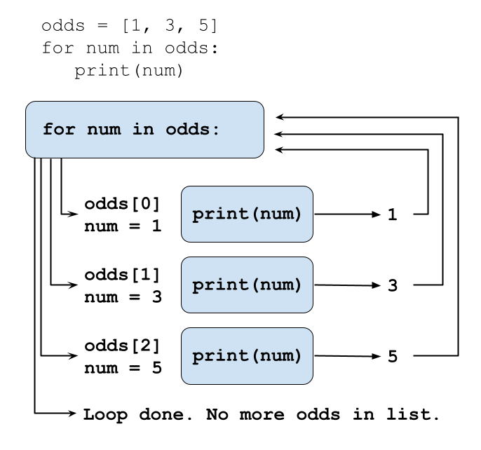
Each number (num) variable in the odds list
is looped through and printed one number after another.
Loop variables
Loop variables are created on demand when you define the loop and
they will persist after the loop finishes. Like all variable names, it’s
helpful to give for loop variables meaningful names that
you’ll understand as the code in your loop grows.
for num in odds is easier to understand than
for kitten in odds, for example.
You can loop through other Python objects
You can use a for loop to iterate through each element
in a string. for loops are not limited to operating on
lists.
OUTPUT
L
i
b
r
a
r
y

o
f

B
a
b
e
l
Use range to iterate over a sequence of numbers.
The built-in function range() produces a sequence of
numbers. You can pass a single parameter to identify how many items in
the sequence to range over (e.g. range(5)) or if you pass
two arguments, the first corresponds to the starting point and the
second to the end point. The end point works in the same way as Python
index values (“up to, but not including”).
OUTPUT
0
1
2
Accumulators
A common loop pattern is to initialize an accumulator variable to zero, an empty string, or an empty list before the loop begins. Then the loop updates the accumulator variable with values from a collection.
We can use the += operator to add a value to
total in the loop below, so that each time we iterate
through the loop we’ll add the index value of the range()
to total.
PYTHON
# Sum the first 10 integers.
total = 0

# range(1,11) will give us the numbers 1 through 10
for num in range(1, 11):
    print(f'num is: {num} total is: {total}')
    total += num

print(f'Loop finished. num is: {num} total is: {total}')
OUTPUT
num is: 1 total is: 0
num is: 2 total is: 1
num is: 3 total is: 3
num is: 4 total is: 6
num is: 5 total is: 10
num is: 6 total is: 15
num is: 7 total is: 21
num is: 8 total is: 28
num is: 9 total is: 36
num is: 10 total is: 45
Loop finished. Num is: 10 total is: 55- The first time through the loop,
totalis equal to 0, andnumis 1 (the range starts at 1). After those values print out we add 1 to the value oftotal(0), to get 1. - The second time through the loop,
totalis equal to 1, andnumis 2. After those print out we add 2 to the value oftotal(1), to get 3. - The third time through the loop,
totalis equal to 3, andnumis 3. After those print out we add 3 to the value oftotal(3), to bring us to 6. - And so on.
- After the loop is finished the values of
totalandnumretain the values that were assigned the last time through the loop. Sonumis equal to 10 (the last index value ofrange()) andtotalis equal to 55 (45 + 10).
Use a string index in a loop
How would you loop through a list with the values ‘red’, ‘green’, and
‘blue’ to create the acronym rgb, pulling from the first
letters in each string? Print the acronym when the loop is finished.
Hint: Use the + operator to concatenate strings
together. For example, lib = 'lib' + 'rary' will assign the
value of ‘library’ to lib.
Subtract a list of values in a loop
- Create an accumulator variable called
totalthat starts at 100. - Create a list called
numberswith the values of 10, 15, 20, 25, 30. - Create a
forloop to iterate through each item in the list. - Each time through the list update the value of
totalto subtract the value of the current list item fromtotal. Tip:-=works for subtraction in the same way that+=works for addition. - Print the value of
totalinside of the loop to keep track of its value throughout.
Key Points
- A for loop executes commands once for each value in a collection.
- The first line of the
forloop must end with a colon, and the body must be indented. - Indentation is always meaningful in Python.
- A
forloop is made up of a collection, a loop variable, and a body. - Loop variables can be called anything (but it is strongly advised to have a meaningful name to the looping variable).
- The body of a loop can contain many statements.
- Use
rangeto iterate over a sequence of numbers. - The Accumulator pattern turns many values into one.
Content from Looping Over Data Sets
Last updated on 2024-05-17 | Edit this page
Overview
Questions
- How can I process many data sets with a single command?
Objectives
- Be able to read and write globbing expressions that match sets of files.
- Use glob to create lists of files.
- Write for loops to perform operations on files given their names in a list.
Use a for loop to process files given a list of their
names.
If you recall from episode 06, the pd.read_csv() method
takes a text string referencing a filename as an argument. If we have a
list of strings that point to our filenames, we can loop through the
list to read in each CSV file as a DataFrame. Let’s print out the
maximum values from the ‘ytd’ (year to date) column for each
DataFrame.
PYTHON
for filename in ['data/2011_circ.csv', 'data/2012_circ.csv']:
  data = pd.read_csv(filename)
  print(filename, data['ytd'].max())
OUTPUT
data/2011_circ.csv 966720
data/2012_circ.csv 937649
Use glob to find sets of files whose names match a
pattern.
Fortunately, we don’t have to manually type in a list of all of our
filenames. We can use a Python library called glob, to work
with paths and files in a convenient way. In Unix, the term “globbing”
means “matching a set of files with a pattern”. Glob gives us some nice
pattern matching options:
-
*will “match zero or more characters” -
?will “match exactly one character”
The glob library contains a function also called
glob to match file patterns. For example,
glob.glob('*.txt') would match all files in the current
directory with names that end with .txt.
Let’s create a list of the usage data CSV files. Because the
.glob() argument includes a filepath in single quotes,
we’ll use double quotes around our f-string.
OUTPUT
all csv files in data directory: ['data/2011_circ.csv', 'data/2016_circ.csv', 'data/2017_circ.csv', 'data/2022_circ.csv', 'data/2018_circ.csv', 'data/2019_circ.csv', 'data/2012_circ.csv', 'data/2013_circ.csv', 'data/2021_circ.csv', 'data/2020_circ.csv', 'data/2015_circ.csv', 'data/2014_circ.csv']Use glob and for to process batches of
files.
Now we can use glob in a for loop to create DataFrames
from all of the CSV files in the data directory. To use
tools like glob it helps if files are named and stored
consistently so that simple patterns will find the right data. You can
learn more about how to name files to improve machine-readability from
the Open Science
Foundation article on file naming.
OUTPUT
data/2011_circ.csv 966720
data/2016_circ.csv 670077
data/2017_circ.csv 634570
data/2022_circ.csv 301340
data/2018_circ.csv 614313
data/2019_circ.csv 581151
data/2012_circ.csv 937649
data/2013_circ.csv 821749
data/2021_circ.csv 271811
data/2020_circ.csv 276878
data/2015_circ.csv 694528
data/2014_circ.csv 755189
The output of the files above may be different for you, depending on
what operating system you use. The glob library doesn’t have its own
internal system for determining how filenames are sorted, but instead
relies on the operating system’s filesystem. Since operating systems can
differ, it is helpful to use Python to manually sort the glob files so
that everyone will see the same results, regardless of their operating
system. You can do that by applying the Python method
sorted() to the glob.glob list.
PYTHON
for csv in sorted(glob.glob('data/*.csv')):
    data = pd.read_csv(csv)
    print(csv, data['ytd'].max())
OUTPUT
data/2011_circ.csv 966720
data/2012_circ.csv 937649
data/2013_circ.csv 821749
data/2014_circ.csv 755189
data/2015_circ.csv 694528
data/2016_circ.csv 670077
data/2017_circ.csv 634570
data/2018_circ.csv 614313
data/2019_circ.csv 581151
data/2020_circ.csv 276878
data/2021_circ.csv 271811
data/2022_circ.csv 301340
Appending DataFrames to a list
In the example above, we can print out results from each DataFrame as we cycle through them, but it would be more convenient if we saved all of the yearly usage data in these CSV files into DataFrames that we could work with later on.
Convert Year in filenames to a column
Before we join the data from each CSV into a single DataFrame, we’ll want to make sure we keep track of which year each dataset comes from. To do that we can capture the year from each file name and save it to a new column for all of the rows in each CSV. Let’s see how this works by looping through each of our CSVs.
PYTHON
for csv in sorted(glob.glob('data/*.csv')):
        year = csv[5:9] #the 5th to 9th characters in each file match the year
        print(f'filename: {csv} year: {year}')
OUTPUT
filename: data/2011_circ.csv year: 2011
filename: data/2012_circ.csv year: 2012
filename: data/2013_circ.csv year: 2013
filename: data/2014_circ.csv year: 2014
filename: data/2015_circ.csv year: 2015
filename: data/2016_circ.csv year: 2016
filename: data/2017_circ.csv year: 2017
filename: data/2018_circ.csv year: 2018
filename: data/2019_circ.csv year: 2019
filename: data/2020_circ.csv year: 2020
filename: data/2021_circ.csv year: 2021
filename: data/2022_circ.csv year: 2022
Once we’ve saved the year variable from each file name,
we can assign it to every row in a column for each CSV by assigning
data['year'] = year inside of the loop.
To collect the data from each CSV we’ll use a list “accumulator” (as we covered in the last episode) and append each DataFrame to an empty list. You can create an empty list by assigning a variable to empty square brackets before the loop begins.
PYTHON
dfs = [] # an empty list to hold all of our DataFrames
counter = 1

for csv in sorted(glob.glob('data/*.csv')):
  year = csv[5:9]
  data = pd.read_csv(csv)
  data['year'] = year
  print(f'{counter} Saving {len(data)} rows from {csv}')
  dfs.append(data)
  counter += 1

print(f'Number of saved DataFrames: {len(dfs)}')
OUTPUT
1 Saving 80 rows from data/2011_circ.csv
2 Saving 79 rows from data/2012_circ.csv
3 Saving 80 rows from data/2013_circ.csv
4 Saving 80 rows from data/2014_circ.csv
5 Saving 80 rows from data/2015_circ.csv
6 Saving 80 rows from data/2016_circ.csv
7 Saving 80 rows from data/2017_circ.csv
8 Saving 80 rows from data/2018_circ.csv
9 Saving 81 rows from data/2019_circ.csv
10 Saving 81 rows from data/2020_circ.csv
11 Saving 81 rows from data/2021_circ.csv
12 Saving 81 rows from data/2022_circ.csv
Number of saved DataFrames: 12
We can check to make sure the year was properly saved by looking at
the first DataFrame in the dfs list. If you scroll to the
right you should see the first two rows of the year column
both have the value 2011.
OUTPUT
|     | branch      | address               | city    | zip code | january | february | march | april | may  | june  | july  | august | september | october | november | december | ytd    | year |
|-----|-------------|-----------------------|---------|----------|---------|----------|-------|-------|------|-------|-------|--------|-----------|---------|----------|----------|--------|------|
| 0   | Albany Park | 5150 N. Kimball Ave.  | Chicago | 60625.0  | 8427    | 7023     | 9702  | 9344  | 8865 | 11650 | 11778 | 11306  | 10466     | 10997   | 10567    | 9934     | 120059 | 2011 |
| 1   | Altgeld     | 13281 S. Corliss Ave. | Chicago | 60827.0  | 1258    | 708      | 854   | 804   | 816  | 870   | 713   | 480    | 702       | 927     | 787      | 692      | 9611   | 2011 |
Concatenating DataFrames
There are many different ways to merge, join, and concatenate pandas
DataFrames together. The pandas
documentation has good examples of how to use the
.merge(), .join(), and .concat()
methods to accomplish different goals. Because all of our CSVs have the
exact same columns, if we want to concatenate them vertically (adding
all of the rows from each DataFrame together in order), we can do so
using concat(), which takes a list of DataFrames as its
first argument. Since we aren’t using a specific column as a pandas
index, we’ll set the argument of ignore_index to be
True.
OUTPUT
'Number of rows in df: 963'Only item 1 is matched by the wildcard expression
data/*circ.csv.
Compile CSVs into one DataFrame
Imagine you had a folder named outputs/ that included
all kinds of different file types. Use glob and a
for loop to iterate through all of the CSV files in the
folder that have a file name that begins with data. Save
them to a list called dfs, and then use
pd.concat() to concatenate all of the DataFrames from the
dfs list together into a new DataFrame called,
new_df. You can assume that all of the data CSV files have
the same columns so they will concatenate together cleanly using
pd.concat().
Key Points
- Use a
forloop to process files given a list of their names. - Use
glob.globto find sets of files whose names match a pattern. - Use
globandforto process batches of files. - Use a list “accumulator” to append a DataFrame to an empty list
[]. - The
.merge(),.join(), and.concat()methods can combine pandas DataFrames.
Content from Using Pandas
Last updated on 2024-05-17 | Edit this page
Overview
Questions
- How can I work with subsets of data in a pandas DataFrame?
- How can I run summary statistics and sort columns of a DataFrame?
- How can I save DataFrames to other file formats?
Objectives
- Select specific columns and rows from pandas DataFrames.
- Use pandas methods to calculate sums and means, and to display unique items.
- Sort DataFrame columns (pandas series).
- Save a DataFrame as a CSV or pickle file.
Pinpoint specific rows and columns in a DataFrame
If you don’t already have all of the CSV files loaded into a DataFrame, let’s do that now:
PYTHON
import glob
import pandas as pd

dfs = []

for csv in sorted(glob.glob('data/*.csv')):
    year = csv[5:9]
    data = pd.read_csv(csv)
    data['year'] = year
    dfs.append(data)

df = pd.concat(dfs, ignore_index=True)

df.head(3)| branch | address | city | zip code | january | february | march | april | may | june | july | august | september | october | november | december | ytd | year | |
|---|---|---|---|---|---|---|---|---|---|---|---|---|---|---|---|---|---|---|
| 0 | Albany Park | 5150 N. Kimball Ave. | Chicago | 60625.0 | 8427 | 7023 | 9702 | 9344 | 8865 | 11650 | 11778 | 11306 | 10466 | 10997 | 10567 | 9934 | 120059 | 2011 |
| 1 | Altgeld | 13281 S. Corliss Ave. | Chicago | 60827.0 | 1258 | 708 | 854 | 804 | 816 | 870 | 713 | 480 | 702 | 927 | 787 | 692 | 9611 | 2011 |
| 2 | Archer Heights | 5055 S. Archer Ave. | Chicago | 60632.0 | 8104 | 6899 | 9329 | 9124 | 7472 | 8314 | 8116 | 9177 | 9033 | 9709 | 8809 | 7865 | 101951 | 2011 |
Use tail() to look at the end of the DataFrame
We’ve seen how to look at the first rows in your DataFrame using
.head(). You can use .tail() to look at the
final rows.
| branch | address | city | zip code | january | february | march | april | may | june | july | august | september | october | november | december | ytd | year | |
|---|---|---|---|---|---|---|---|---|---|---|---|---|---|---|---|---|---|---|
| 960 | Brighton Park | 4314 S. Archer Ave. | Chicago | 60632.0 | 1394 | 1321 | 1327 | 1705 | 1609 | 1578 | 1609 | 1512 | 1425 | 1603 | 1579 | 1278 | 17940 | 2022 |
| 961 | South Chicago | 9055 S. Houston Ave. | Chicago | 60617.0 | 496 | 528 | 739 | 775 | 587 | 804 | 720 | 883 | 681 | 697 | 799 | 615 | 8324 | 2022 |
| 962 | Chicago Bee | 3647 S. State St. | Chicago | 60609.0 | 799 | 543 | 709 | 803 | 707 | 931 | 778 | 770 | 714 | 835 | 718 | 788 | 9095 | 2022 |
Slicing a DataFrame
We can use the same slicing syntax that we used for strings and lists to look at a specific range of rows in a DataFrame.
| branch | address | city | zip code | january | february | march | april | may | june | july | august | september | october | november | december | ytd | year | |
|---|---|---|---|---|---|---|---|---|---|---|---|---|---|---|---|---|---|---|
| 50 | Near North | 310 W. Division St. | Chicago | 60610.0 | 11032 | 10021 | 12911 | 12621 | 12437 | 13988 | 13955 | 14729 | 13989 | 13355 | 13006 | 12194 | 154238 | 2011 |
| 51 | North Austin | 5724 W. North Ave. | Chicago | 60639.0 | 2481 | 2045 | 2674 | 2832 | 2202 | 2694 | 3302 | 3225 | 3160 | 3074 | 2796 | 2272 | 32757 | 2011 |
| 52 | North Pulaski | 4300 W. North Ave. | Chicago | 60639.0 | 3848 | 3176 | 4111 | 5066 | 3885 | 5105 | 5916 | 5512 | 5349 | 6386 | 5952 | 5372 | 59678 | 2011 |
| 53 | Northtown | 6435 N. California Ave. | Chicago | 60645.0 | 10191 | 8314 | 11569 | 11577 | 10902 | 14202 | 15310 | 14152 | 11623 | 12266 | 12673 | 12227 | 145006 | 2011 |
| 54 | Oriole Park | 7454 W. Balmoral Ave. | Chicago | 60656.0 | 11999 | 11206 | 13675 | 12755 | 10364 | 12781 | 12219 | 12066 | 10856 | 11324 | 10503 | 9878 | 139626 | 2011 |
| 55 | Portage-Cragin | 5108 W. Belmont Ave. | Chicago | 60641.0 | 9185 | 7634 | 9760 | 10163 | 7995 | 9735 | 10617 | 11203 | 10188 | 11418 | 10718 | 9517 | 118133 | 2011 |
| 56 | Pullman | 11001 S. Indiana Ave. | Chicago | 60628.0 | 1916 | 1206 | 1975 | 2176 | 2019 | 2347 | 2092 | 2426 | 2476 | 2611 | 2530 | 2033 | 25807 | 2011 |
| 57 | Roden | 6083 N. Northwest Highway | Chicago | 60631.0 | 6336 | 5830 | 7513 | 6978 | 6180 | 8519 | 8985 | 7592 | 6628 | 7113 | 6999 | 6082 | 84755 | 2011 |
| 58 | Rogers Park | 6907 N. Clark St. | Chicago | 60626.0 | 10537 | 9683 | 13812 | 13745 | 13368 | 18314 | 20367 | 19773 | 18419 | 18972 | 17255 | 16597 | 190842 | 2011 |
| 59 | Roosevelt | 1101 W. Taylor St. | Chicago | 60607.0 | 6357 | 6171 | 8228 | 7683 | 7257 | 8545 | 8134 | 8289 | 7696 | 7598 | 7019 | 6665 | 89642 | 2011 |
Look at specific columns
To work specifically with one column of a DataFrame we can use a similar syntax, but refer to the name the column of interest.
OUTPUT
0      2011
1      2011
2      2011
3      2011
4      2011
       ...
958    2022
959    2022
960    2022
961    2022
962    2022
Name: year, Length: 963, dtype: object
We can add a second square bracket after a column name to refer to specific row indices, either on their own, or using slices to look at ranges.
PYTHON
print(f"first row: {df['year'][0]}") #use double quotes around your fstring if it contains single quotes
print('rows 100 to 102:') #add a new print statement to create a new line
print(df['year'][100:103])
OUTPUT
first row: 2011
rows 100 to 102:
100    2012
101    2012
102    2012
Name: year, dtype: object
Columns display differently in our notebook since a column is a different type of object than a full DataFrame.
OUTPUT
pandas.core.series.SeriesSummary statistics on columns
A pandas Series is a one-dimensional array, like a column in a
spreadsheet, while a pandas DataFrame is a two-dimensional tabular data
structure with labeled axes, similar to a spreadsheet. One of the
advantages of pandas is that we can use built-in functions like
max(), min(), mean(), and
sum() to provide summary statistics across Series such as
columns. Since it can be difficult to get a sense of the range of data
in a large DataFrame by looking over the whole thing manually, these
functions can help us understand our dataset quickly and ask specific
questions.
If we wanted to know the range of years covered in this data, for
example, we can look at the maximum and minimum values in the
year column.
OUTPUT
max year: 2022
min year: 2011
Summarize columns that hold string objects
We might also want to quickly understand the range of values in
columns that contain strings, the branch column, for
example. We can look at a range of values, but it’s hard to tell how
many different branches are present in the dataset this way.
OUTPUT
0         Albany Park
1             Altgeld
2      Archer Heights
3              Austin
4       Austin-Irving
            ...
958         Chinatown
959          Brainerd
960     Brighton Park
961     South Chicago
962       Chicago Bee
Name: branch, Length: 963, dtype: object
We can use the .unique() function to output an array
(like a list) of all of the unique values in the branch
column, and the .nunique() function to tell us how many
unique values are present.
OUTPUT
Number of unique branches: 82
['Albany Park' 'Altgeld' 'Archer Heights' 'Austin' 'Austin-Irving'
 'Avalon' 'Back of the Yards' 'Beverly' 'Bezazian' 'Blackstone' 'Brainerd'
 'Brighton Park' 'Bucktown-Wicker Park' 'Budlong Woods' 'Canaryville'
 'Chicago Bee' 'Chicago Lawn' 'Chinatown' 'Clearing' 'Coleman'
 'Daley, Richard J. - Bridgeport' 'Daley, Richard M. - W Humboldt'
 'Douglass' 'Dunning' 'Edgebrook' 'Edgewater' 'Gage Park'
 'Galewood-Mont Clare' 'Garfield Ridge' 'Greater Grand Crossing' 'Hall'
 'Harold Washington Library Center' 'Hegewisch' 'Humboldt Park'
 'Independence' 'Jefferson Park' 'Jeffery Manor' 'Kelly' 'King'
 'Legler Regional' 'Lincoln Belmont' 'Lincoln Park' 'Little Village'
 'Logan Square' 'Lozano' 'Manning' 'Mayfair' 'McKinley Park' 'Merlo'
 'Mount Greenwood' 'Near North' 'North Austin' 'North Pulaski' 'Northtown'
 'Oriole Park' 'Portage-Cragin' 'Pullman' 'Roden' 'Rogers Park'
 'Roosevelt' 'Scottsdale' 'Sherman Park' 'South Chicago' 'South Shore'
 'Sulzer Regional' 'Thurgood Marshall' 'Toman' 'Uptown' 'Vodak-East Side'
 'Walker' 'Water Works' 'West Belmont' 'West Chicago Avenue'
 'West Englewood' 'West Lawn' 'West Pullman' 'West Town'
 'Whitney M. Young, Jr.' 'Woodson Regional' 'Wrightwood-Ashburn'
 'Little Italy' 'West Loop']
Use .groupby() to analyze subsets of data
A reasonable question to ask of the library usage data might be to
see which branch library has seen the most checkouts over this ten +
year period. We can use .groupby() to create subsets of
data based on the values in specific columns. For example, let’s group
our data by branch name, and then look at the ytd column to
see which branch has the highest usage. .groupby() takes a
column name as its argument and then for each group we can sum the
ytd columns using .sum().
OUTPUT
branch
Albany Park              1024714
Altgeld                    68358
Archer Heights            803014
Austin                    200107
Austin-Irving            1359700
                          ...
West Pullman              295327
West Town                 922876
Whitney M. Young, Jr.     259680
Woodson Regional          823793
Wrightwood-Ashburn        302285
Name: ytd, Length: 82, dtype: int64
Sort pandas series using .sort_values()
The output for code above is another pandas series object. Let’s save
the output to a new variable so we can then apply the
.sort_values() method which allows us to view the branches
with the most usage. The ascending parameter for
.sort_values() takes True or
False. We want to pass False so that we sort
from the highest values down…
PYTHON
circ_by_branch = df.groupby('branch')['ytd'].sum()
circ_by_branch.sort_values(ascending=False).head(10)
OUTPUT
branch
Harold Washington Library Center    7498041
Sulzer Regional                     5089225
Lincoln Belmont                     1850964
Edgewater                           1668693
Logan Square                        1539816
Rogers Park                         1515964
Bucktown-Wicker Park                1456669
Lincoln Park                        1441173
Austin-Irving                       1359700
Bezazian                            1357922
Name: ytd, dtype: int64
Now we have a list of the branches with the highest number of uses across the whole dataset.
We can pass multiple columns to groupby() to subset the
data even further and breakdown the highest usage per year and branch.
To do that, we need to pass the column names as a list. We can also
chain together many methods into a single line of code.
PYTHON
circ_by_year_branch = df.groupby(['year', 'branch'])['ytd'].sum().sort_values(ascending=False)
circ_by_year_branch.head(5)
OUTPUT
year  branch
2011  Harold Washington Library Center    966720
2012  Harold Washington Library Center    937649
2013  Harold Washington Library Center    821749
2014  Harold Washington Library Center    755189
2015  Harold Washington Library Center    694528
Name: ytd, dtype: int64
Use .iloc[] and .loc[] to select DataFrame locations.
You can point to specific locations in a DataFrame using
two-dimensional numerical indexes with .iloc[].
PYTHON
# print values in the 1st and 2nd to last columns in the first row
# '\n' prints a linebreak
print(f"Branch: {df.iloc[0,0]} \nYTD circ: {df.iloc[0,-2]}")
OUTPUT
Branch: Albany Park
YTD circ: 120059
.loc[] uses the same structure but takes row (index) and
column names instead of numerical indexes. Since our df
rows don’t have index names we would still use the default numerical
index.
PYTHON
# print the same values as above, using the column names
print(f"Branch: {df.loc[0,'branch']} \nYTD circ: {df.loc[0, 'ytd']}")
OUTPUT
Branch: Albany Park
YTD circ: 120059
Save DataFrames
You might want to export the series of usage by year and branch that
we just created so that you can share it with colleagues. Pandas
includes a variety of methods that begin with .to_... that
allow us to convert and export data in different ways. First, let’s save
our series as a DataFrame so we can view the output in a better format
in our Jupyter notebook.
| ytd | ||
|---|---|---|
| year | branch | |
| 2011 | Harold Washington Library Center | 966720 |
| 2012 | Harold Washington Library Center | 937649 |
| 2013 | Harold Washington Library Center | 821749 |
| 2014 | Harold Washington Library Center | 755189 |
| 2015 | Harold Washington Library Center | 694528 |
Save to CSV
Next, let’s export the new DataFrame to a CSV file so we can share it
with colleagues who love spreadsheets. The .to_csv() method
expects a string that will be the name of the file as a parameter. Make
sure to add the .csv filetype to your file name.
You should now see, in the JupyterLab file explorer to the left, the new CSV file. If you don’t see it, you can hit the refresh icon (it looks like a spinning arrow) above the files pane. You can double-click on the CSV to preview the full spreadsheet in a new Jupyter tab.
Save pickle files
Working with your data in CSVs (especially via tools like Microsoft Excel) can introduce reproducibility issues. For example, you’ll sometimes encounter character encoding problems, where certain characters in your dataset will no longer display properly after editing them in a spreadsheet software like Excel, and re-importing them to a pandas DataFrame.
One way to avoid issues like this is to save Python objects as pickles. Technically speaking, the Python pickle module serializes and de-serializes a Python object’s structure. In practical terms, pickling allows you to store Python objects (like DataFrames, lists, etc.) efficiently and without losing or corrupting your data.
You can save a DataFrame to pickle by using the
to_pickle() method and using the filetype of
pkl.
You can only “see” the data in a pickle file by reloading it into Python. This is a great way to save a DataFrame that you created in one JupyterLab session so that you can reload it later on, or share it with a colleague who’s familiar with Python.
Finally, let’s save our full concatenated DataFrame to a pickle file
that we can use later on in the lesson. We’ll save it in the
data/ directory alongside our other data files.
Summary statistics and groupby()
We can apply mean() to pandas series’ in the same way we
used sum(), min(), and max()
above. How would you display the following?
- the mean number of ytd checkouts grouped by zip code?
- the mean number of ytd checkouts grouped by zip code, and sorted from smallest to largest?
Key Points
- Use builtin methods
.sum(),.mean(),unique(), andnunique()to explore summary statistics on the rows and colums in your DataFrame. - Use
.groupby()to work with subsets of your dataset. - Sort pandas series with
.sort_values(). - Use
.loc()and.iloc()to pinpoint specific locations in Pandas DataFrames. - Save DataFrames to CSV and pickle files using
.to_csv()and.to_pickle().
Content from Conditionals
Last updated on 2024-05-08 | Edit this page
Overview
Questions
- How can programs do different things for different data?
Objectives
- Correctly write programs that use
ifandelsestatements using Boolean expressions. - Trace the execution of conditionals inside of loops.
Use if statements to control whether or not a block of
code is executed.
An if statement is a conditional statement that
controls whether a block of code is executed or not. The syntax of an
if statement is similar to a for
statement:
- The first line opens with
ifand ends with a colon. - The body is indented (usually by 4 spaces)
PYTHON
checkouts = 11
if checkouts > 10.0:
    print(f'{checkouts} is over the limit.')

checkouts = 8
if checkouts > 10.0:
    print(f'{checkouts} is over the limit.')
OUTPUT
11 is over the limit.Conditionals are often used inside loops.
There is not much of a point using a conditional when we know the value (as above), but they’re useful when we have a collection to process.
PYTHON
checkouts = [0, 3, 10, 12, 22]
for checkout in checkouts:
    if checkout > 10.0:
        print(f'{checkout} is over the limit.')
OUTPUT
12 is over the limit.
22 is over the limit.
Use else to execute a block of code when an
if condition is not true.
An else statement can be used following if
to allow us to specify an alternative code block to execute when the
if branch is not taken.
PYTHON
for checkout in checkouts:
    if checkout > 10.0:
        print(f'{checkout} is over the limit.')
    else:
        print(f'{checkout} is under the limit.')
OUTPUT
0 is under the limit.
3 is under the limit.
10 is under the limit.
12 is over the limit.
22 is over the limit.
Notice that our else statement led to a false output
that says 10 is under the limit. We can address this by adding a
different kind of else statement.
Use elif to specify additional tests.
You can use elif (short for “else if”) to provide
several alternative choices, each with its own test. An
elif statement should always be associated with an
if statement, and must come before the else
statement (which is the catch all).
PYTHON
for checkout in checkouts:
    if checkout > 10.0:
        print(f'*Warning*: {checkout} is over the limit.')
    elif checkout == 10:
        print(f'{checkout} is at the exact limit.')
    else:
        print(f'{checkout} is under the limit.')
OUTPUT
0 is under the limit.
3 is under the limit.
10 is at the exact limit.
*Warning*: 12 is over the limit.
*Warning*: 22 is over the limit.
Conditions are tested once, in order and are not re-evaluated if values change. Python steps through the branches of the conditional in order, testing each in turn, so the order of your statements matters.
PYTHON
grade = 85
if grade >= 70:
    print('grade is C')
elif grade >= 80:
    print('grade is B')
elif grade >= 90:
    print('grade is A')
OUTPUT
grade is CCompound conditionals using and and
or
Often, you want some combination of things to be true. You can
combine relations within a conditional using and and
or.
We can also check if something is less/greater than or equal to a
value by using >= and <= operators.
PYTHON
checkouts = [3, 50, 120]
users = ['fac', 'grad']

for user in users:
    for checkout in checkouts:
        #faculty checkout limit is 100
        if checkout >= 100 and user == 'fac':
            print(f"*Warning*: {checkout} is over the {user} limit.")

        #grad limit is 50
        elif checkout >= 50 and user == 'grad':
            print(f"{checkout} is over the {user} limit.")

        else:
            print(f"{checkout} is under the {user} limit.")

    # print an empty line between users
    print()
OUTPUT
3 is under the fac limit.
50 is under the fac limit.
*Warning*: 120 is over the fac limit.

3 is under the grad limit.
*Warning*: 50 is over the grad limit.
*Warning*: 120 is over the grad limit.
Age conditionals
Write a Python program that checks the age of a user to determine if they will receive a youth or adult library card. The program should:
- Store
agein a variable. - Use an
ifstatement to check if the age is 16 or older. If true, print “You are eligible for an adult library card.” - Use an
elsestatement to print “You are eligible for a youth library card” if the age is less than 16.
If you finish early, try this challenge:
- In a new cell, adapt your program to loop through a list of age values, testing each age with the same output as above.
Conditional logic: Fill in the blanks
Fill in the blanks in the following program to check if both the name variable is present in the names list and the password variable is equal to ‘true’ before giving a user access to a library system.
If you have extra time after you solve the fill in the blanks, change
the value of password and re-run the program to view the
output.
PYTHON
names = ['Wang', 'Garcia', 'Martin']
name = 'Martin'
password = 'true'

___ item in names:
    print(item)
    if name == item ___ password == _____:
        print('Login successful!')
    elif password __ 'true':
        print(f'Your password is incorrect. Try again.')
    ____ name __ item:
        print(f'- Name does not match. Testing the next item in the list for {name}...')
PYTHON
names = ['Wang', 'Garcia', 'Martin']
name = 'Martin'
password = 'true'

for item in names:
    print(item)
    if name == item and password == 'true':
        print('Login successful!')
    elif password != 'true':
        print(f'Your password is incorrect. Try again.')
    elif name != item:
        print(f'- Name does not match. Testing the next item in the list for {name}...')
OUTPUT
Wang
- Name does not match. Testing the next item in the list for Martin...
Garcia
- Name does not match. Testing the next item in the list for Martin...
Martin
Login successful!Key Points
- Use
ifstatements to control whether or not a block of code is executed. - Conditionals are often used inside loops.
- Use
elseto execute a block of code when anifcondition is not true. - Use
elifto specify additional tests. - Conditions are tested once, in order.
- Use
andandorto check against multiple value statements.
Content from Writing Functions
Last updated on 2024-05-10 | Edit this page
Overview
Questions
- How can I create my own functions?
- How do variables inside and outside of functions work?
- How can I make my functions easier to understand?
Objectives
- Explain and identify the difference between function definition and function call.
- Write a function that takes a small, fixed number of arguments and produces a single result.
- Identify local and global variables.
Use functions to make your code easier to understand.
Human beings can only keep a few items in working memory at a time. But we can work with larger and more complicated ideas by breaking content down into pieces. Functions serve a similar purpose in Python. We can create our own functions to encapsulate complexity and treat specific actions or ideas as a single “thing”. Functions also enable us to re-use code so we can write code one time, but use it many times.
Define a function using def with a name, parameters,
and a block of code.
Begin each definition of a new function with the keyword
def (for “define”), followed by the name of the function.
Function names follow the same rules as variable names. Next, add your
parameters in parentheses. You should still use empty
parentheses if the function doesn’t take any inputs. Finally, like in
conditionals and loops, you’ll add a colon and an indented block of code
that will contain the body of your function.
Defining a function does not run it.
Note that we don’t have any output when we run code to define a function. This is similar to assigning a value to a variable. The function definition is sort of like a recipe in a cookbook - the recipe doesn’t create a meal until we use it. So we need to “call” a function to execute the code it contains. This means that Python won’t show you errors in your function until you call it. So when a definition of a function runs without error it doesn’t mean that there won’t be errors when it executes later.
OUTPUT
Hello!Arguments in call are matched to parameters in definition.
Functions are highly useful when they use parameters to pull in data. You can specify parameters when you define a function which become variables when the function is executed.
PYTHON
def print_date(year, month, day):
    joined = f'{year}/{month}/{day}'
    print(joined)

print_date(1871, 3, 19)
OUTPUT
1871/3/19To expand on the recipe metaphor above, the arguments you add to the
() contain the ingredients for the function, while the body
contains the recipe.
Functions with defined parameters will result in an error if they are called without passing an argument:
ERROR
TypeError                                 Traceback (most recent call last)
Cell In[15], line 1
----> 1 print_date()

TypeError: print_date() missing 3 required positional arguments: 'year', 'month', and 'day'
Use return to pass values back from a function.
In the date example above, we printed the results of the function
code to output, but there are better way to handle data and objects
created within a function. We can use the keyword
return ... to send a value back to the “global”
environment. (We’ll learn about local and global variables below). A
return command can occur anywhere in the function, but is often placed
at the very end of a function with the final result.
PYTHON
def calc_fine(days_overdue):
    if days_overdue <= 10:
        fine =  days_overdue * 0.25
    else:
        fine = (days_overdue * 0.25) + (days_overdue * .50)
    return fine

fine = calc_fine(12)
f'Fine owed: ${fine}'
OUTPUT
'Fine owed: $9.0'Specify the number of float decimals to display
In the example above, the fine value is displayed as
9.0, though ideally it would print as $9.00.
We can use the f-string format specifier of
.2f to display two decimal points: {fine:.2f}.
If you wanted to display a float with three decimal points you would
change the format specifier to {fine:.3f}. Here’s a cheat sheet of other f-string number
formats.
OUTPUT
'Fine owed: $9.00'A function that doesn’t explicitly return a value will
automatically return None.
OUTPUT
1970/6/21
result of call is: None
Variable scope
When we define a variable inside of a function in Python, it’s known
as a local variable, which means that it’s not visible to –
or known by – the rest of the program. Variables that we define outside
of functions are global and are therefore visible
throughout the program, including from within other functions.
The part of a program in which a variable is visible is called its
scope.
This is helpful for people using or writing functions, because they don’t need to worry about repeating variable names that have been created elsewhere in the program.
PYTHON
initial_fine = 0.25
late_fine = 0.50

def calc_fine(days_overdue):
    if days_overdue <= 10:
        days_overdue =  days_overdue * initial_fine
    else:
        days_overdue = (days_overdue * initial_fine) + (days_overdue * late_fine)
    return days_overdue
-
initial_fineandlate_fineare global variables. -
days_overdueis a local variable incalc_fine. Note that a function parameter is a variable that is automatically assigned a value when the function is called and so acts as a local variable.
PYTHON
fine = calc_fine(12)
print(f'Fine owed: ${fine:.2f}')
print(f'Fine rates: ${initial_fine:.2f}, ${late_fine:.2f}')
print(f'Days overdue: {days_overdue}')
OUTPUT
Fine owed: $9.00
Fine rates: $0.25, $0.50
ERROR
NameError                                 Traceback (most recent call last)
Cell In[22], line 4
      2 print(f'Fine owed: ${fine:.2f}')
      3 print(f'Fine rates: ${initial_fine:.2f}, ${late_fine:.2f}')
----> 4 print(f'Days overdue: {days_overdue}')

NameError: name 'days_overdue' is not defined
Use docstrings to provide online help.
If the first thing in a function is a string that isn’t assigned to a
variable, that string is attached to the function as its documentation.
This kind of documentation at the beginning of a function is called a
docstring.
PYTHON
def fahr_to_celsius(temp):
    "Input a fahrenheit temperature and return the value in celsius"
    return ((temp - 32) * (5/9))
This is helpful because we can now ask Python’s built-in help system to show us the documentation for the function:
OUTPUT
Help on function fahr_to_celsius in module __main__:

fahr_to_celsius(temp)
    Input a fahrenheit temperature and return the value in celsius
We don’t need to use triple quotes when we write a docstring, but if we do, we can break the string across multiple lines:
PYTHON
def fahr_to_celsius(temp):
    """Convert fahrenheit values to celsius
    Input a value in fahrenheit
    Output a value in celsius"""
return ((temp - 32) * (5/9))Conditional statements within functions
Create a function called grade_converter that takes a
numerical score (0 - 100) as its parameter and returns a letter grade
based on the score:
- 90 and above returns ‘A’
- 80 to 89 returns ‘B’
- 70 to 79 returns ‘C’
- 60 to 69 returns ‘D’
- Below 60 returns ‘F’
After defining the function, test it with a variety of scores to test it out.
Local and global variables
List all of the global variables and all of the local variables in the following code.
PYTHON
fine_rate = 0.25

def fine(days_overdue):
    if days_overdue <= 10:
        fine =  days_overdue * fine_rate
    else:
        fine = (days_overdue * fine_rate) + (days_overdue * (fine_rate*2))
    return fine

total_fine = calc_fine(20)
f'Fine owed: ${total_fine:.2f}'
OUTPUT
'Fine owed: $15.00'Global variables:
- fine_rate
- total_fine
Local variables:
- days_overdue
- fine
CSVs to Pandas function
In the Looping Data Sets episode, we learned to use glob to loop through a directory of CSV files and convert them to a Pandas DataFrame.
Write a function that converts a directory of CSV files into a single
Pandas DataFrame. The function should accept one parameter: a string
that includes the path and glob wildcard expression to point to a set of
CSV files (e.g., 'data/*.csv'). We can assume, for these
purposes, that all of the DataFrames have the same column names so that
you can use pd.concat(dfs, ignore_index=True) at the end of
the function to concatenate a list of DataFrames into a single
DataFrame.
Key Points
- Break programs down into functions to make them easier to understand.
- Define a function using
defwith a name, parameters, and a block of code. - Defining a function does not run it.
- Arguments in call are matched to parameters in definition.
- Functions may return a result to their caller using
return.
Content from Tidy Data with Pandas
Last updated on 2024-06-14 | Edit this page
Overview
Questions
- What are the benefits of transforming data into a tidy format for analysis?
- How does the melt() function in pandas facilitate data tidying?
- What are some practical challenges when working with real-world datasets in Python, and how can they be addressed?
Objectives
- Identify the characteristics of tidy data and explain its benefits, listing the three principles and discussing how it facilitates data analysis during a review session.
- Use pandas functions like concat(), melt(), and data filtering to manipulate and clean a complex dataset, successfully combining multiple files into a single DataFrame and reshaping it using melt()
Tidy Data in Pandas
Let’s import the pickle file that contains all of our Chicago public
library circulation data in a single DataFrame. We can use the Pandas
.read_pickle() method to do so.
| branch | address | city | zip code | january | february | march | april | may | june | july | august | september | october | november | december | ytd | year | |
|---|---|---|---|---|---|---|---|---|---|---|---|---|---|---|---|---|---|---|
| 0 | Albany Park | 5150 N. Kimball Ave. | Chicago | 60625.0 | 8427 | 7023 | 9702 | 9344 | 8865 | 11650 | 11778 | 11306 | 10466 | 10997 | 10567 | 9934 | 120059 | 2011 |
| 1 | Altgeld | 13281 S. Corliss Ave. | Chicago | 60827.0 | 1258 | 708 | 854 | 804 | 816 | 870 | 713 | 480 | 702 | 927 | 787 | 692 | 9611 | 2011 |
| 2 | Archer Heights | 5055 S. Archer Ave. | Chicago | 60632.0 | 8104 | 6899 | 9329 | 9124 | 7472 | 8314 | 8116 | 9177 | 9033 | 9709 | 8809 | 7865 | 101951 | 2011 |
| 3 | Austin | 5615 W. Race Ave. | Chicago | 60644.0 | 1755 | 1316 | 1942 | 2200 | 2133 | 2359 | 2080 | 2405 | 2417 | 2571 | 2233 | 2116 | 25527 | 2011 |
| 4 | Austin-Irving | 6100 W. Irving Park Rd. | Chicago | 60634.0 | 12593 | 11791 | 14807 | 14382 | 11754 | 14402 | 14605 | 15164 | 14306 | 15357 | 14069 | 12404 | 165634 | 2011 |
| branch | address | city | zip code | january | february | march | april | may | june | july | august | september | october | november | december | ytd | year | |
|---|---|---|---|---|---|---|---|---|---|---|---|---|---|---|---|---|---|---|
| 958 | Chinatown | 2100 S. Wentworth Ave. | Chicago | 60616.0 | 4795 | 4258 | 5316 | 5343 | 4791 | 5367 | 5477 | 5362 | 4991 | 4847 | 4035 | 3957 | 58539 | 2022 |
| 959 | Brainerd | 1350 W. 89th St. | Chicago | 60620.0 | 255 | 264 | 370 | 386 | 399 | 421 | 337 | 373 | 361 | 276 | 256 | 201 | 3899 | 2022 |
| 960 | Brighton Park | 4314 S. Archer Ave. | Chicago | 60632.0 | 1394 | 1321 | 1327 | 1705 | 1609 | 1578 | 1609 | 1512 | 1425 | 1603 | 1579 | 1278 | 17940 | 2022 |
| 961 | South Chicago | 9055 S. Houston Ave. | Chicago | 60617.0 | 496 | 528 | 739 | 775 | 587 | 804 | 720 | 883 | 681 | 697 | 799 | 615 | 8324 | 2022 |
| 962 | Chicago Bee | 3647 S. State St. | Chicago | 60609.0 | 799 | 543 | 709 | 803 | 707 | 931 | 778 | 770 | 714 | 835 | 718 | 788 | 9095 | 2022 |
Let’s take a moment to discuss the setup of our DataFrame. It is structured in what is known as a wide format. This format displays an extensive amount of data directly on the screen, with each month’s circulation counts spread across the columns in a pivoted manner. This layout makes it easier to read and manually manipulate the data in a spreadsheet and because of this, is often the default output for periodic reporting systems like integrated library systems.
However, this wide format can pose challenges when working with data analysis tools like Pandas. For instance, if we need to identify all the library branches where circulation exceeded 10,000 in any given month, we would have to individually check each column dedicated to a month, which can be quite cumbersome.
To address this we can reshape our data in a long format. This is sometimes called un-pivoting the data, and in our case the month columns will become a single variable in the dataset.
Tidy Data
Tidy data is a standard way of organizing data values within a dataset, making it easier to work with. Here are the key principles of tidy data: 1. Every column holds a single variable, like “month” or “temperature.” 2. Every row represents a single observation, like circulation counts by branch and month. 3. Every cell contains a single value.
The image below might help orient us to the concept of tidy data.
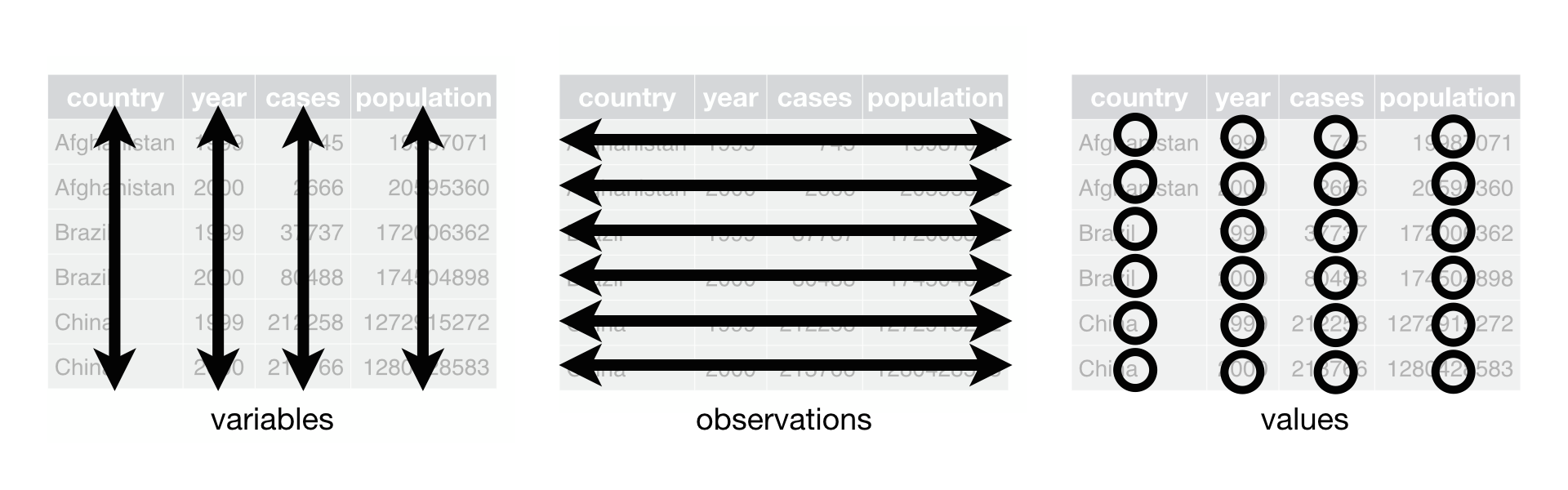
R for Data Science 12.1
Benefits of Tidy Data
Transforming our data into a tidy data format provides several advantages: - Python operations, such as visualization, filtering, and statistical analysis libraries, work better with data in a tidy format. - Tidy data makes transforming, summarizing, and visualizing information easier. For instance, comparing monthly trends or calculating annual averages becomes more straightforward. - As datasets grow, tidy data ensures that they remain manageable and analyses remain accurate.
Making Our Data Tidy
A good step towards tidying our data would be to consolidate the
separate month columns into a column called month, and the
circulation counts into another column called
circulation_counts. This simplifies our data and aligns
with the principles of tidy data.
To achieve this transformation, we can use a Pandas function called
melt(). This function reshapes the data from wide to long
format, where each row will represent one month’s circulation data for a
branch. Let’s look at the help for melt first.
Now, let’s tidy our data. We’ll create a new dataframe called
df_long and use melt to reshape.
melt essentially melts down our columns into rows.
PYTHON
df_long = df.melt(id_vars=['branch', 'address', 'city', 'zip code', 'ytd', 'year'],
                    value_vars=['january', 'february', 'march', 'april', 'may', 'june',
                                'july', 'august', 'september', 'october', 'november', 'december'],
                    var_name='month', value_name='circulation')
In the above code we use id_vars to list the columns we
do not want to melt. We then identify the columns we do want to melt
into rows in the value_vars parameter.
var_name is the variable name for the columns that will be
transformed into rows. value_names is the measured
variable, circulation in our case. Let’s now look at the
new structure of our data.
| branch | address | city | zip code | ytd | year | month | circulation | |
|---|---|---|---|---|---|---|---|---|
| 0 | Albany Park | 5150 N. Kimball Ave. | Chicago | 60625.0 | 120059 | 2011 | january | 8427 |
| 1 | Altgeld | 13281 S. Corliss Ave. | Chicago | 60827.0 | 9611 | 2011 | january | 1258 |
| 2 | Archer Heights | 5055 S. Archer Ave. | Chicago | 60632.0 | 101951 | 2011 | january | 8104 |
| 3 | Austin | 5615 W. Race Ave. | Chicago | 60644.0 | 25527 | 2011 | january | 1755 |
| 4 | Austin-Irving | 6100 W. Irving Park Rd. | Chicago | 60634.0 | 165634 | 2011 | january | 12593 |
| … | … | … | … | … | … | … | … | … |
| 11551 | Chinatown | 2100 S. Wentworth Ave. | Chicago | 60616.0 | 58539 | 2022 | december | 3957 |
| 11552 | Brainerd | 1350 W. 89th St. | Chicago | 60620.0 | 3899 | 2022 | december | 201 |
| 11553 | Brighton Park | 4314 S. Archer Ave. | Chicago | 60632.0 | 17940 | 2022 | december | 1278 |
| 11554 | South Chicago | 9055 S. Houston Ave. | Chicago | 60617.0 | 8324 | 2022 | december | 615 |
| 11555 | Chicago Bee | 3647 S. State St. | Chicago | 60609.0 | 9095 | 2022 | december | 788 |
Ok, let’s look at the unique branches in our long DataFrame:
OUTPUT
array(['Albany Park', 'Altgeld', 'Archer Heights', 'Austin',
       'Austin-Irving', 'Avalon', 'Back of the Yards', 'Beverly',
       'Bezazian', 'Blackstone', 'Brainerd', 'Brighton Park',
       'Bucktown-Wicker Park', 'Budlong Woods', 'Canaryville',
       'Chicago Bee', 'Chicago Lawn', 'Chinatown', 'Clearing', 'Coleman',
       'Daley, Richard J. - Bridgeport', 'Daley, Richard M. - W Humboldt',
       'Douglass', 'Dunning', 'Edgebrook', 'Edgewater', 'Gage Park',
       'Galewood-Mont Clare', 'Garfield Ridge', 'Greater Grand Crossing',
       'Hall', 'Harold Washington Library Center', 'Hegewisch',
       'Humboldt Park', 'Independence', 'Jefferson Park', 'Jeffery Manor',
       'Kelly', 'King', 'Legler Regional', 'Lincoln Belmont',
       'Lincoln Park', 'Little Village', 'Logan Square', 'Lozano',
       'Manning', 'Mayfair', 'McKinley Park', 'Merlo', 'Mount Greenwood',
       'Near North', 'North Austin', 'North Pulaski', 'Northtown',
       'Oriole Park', 'Portage-Cragin', 'Pullman', 'Roden', 'Rogers Park',
       'Roosevelt', 'Scottsdale', 'Sherman Park', 'South Chicago',
       'South Shore', 'Sulzer Regional', 'Thurgood Marshall', 'Toman',
       'Uptown', 'Vodak-East Side', 'Walker', 'Water Works',
       'West Belmont', 'West Chicago Avenue', 'West Englewood',
       'West Lawn', 'West Pullman', 'West Town', 'Whitney M. Young, Jr.',
       'Woodson Regional', 'Wrightwood-Ashburn', 'Little Italy',
       'West Loop'], dtype=object)
Alright! Now that we have the data tidied what can we do with it?
Let’s look at which branches circulated over 10,000 items in any given
month. We can filter the df_long DataFrame to only show
rows that have a number greater than 10,000 in the
circulation column.
| branch | address | city | zip code | ytd | year | month | circulation | |
|---|---|---|---|---|---|---|---|---|
| 4 | Austin-Irving | 6100 W. Irving Park Rd. | Chicago | 60634.0 | 165634 | 2011 | january | 12593 |
| 12 | Bucktown-Wicker Park | 1701 N. Milwaukee Ave. | Chicago | 60647.0 | 173396 | 2011 | january | 13113 |
| 13 | Budlong Woods | 5630 N. Lincoln Ave. | Chicago | 60659.0 | 160271 | 2011 | january | 12841 |
| 17 | Chinatown | 2353 S. Wentworth Ave. | Chicago | 60616.0 | 158449 | 2011 | january | 14027 |
| 24 | Edgebrook | 5331 W. Devon Ave. | Chicago | 60646.0 | 129288 | 2011 | january | 10231 |
| … | … | … | … | … | … | … | … | … |
| 11373 | Harold Washington Library Center | 400 S. State St. | Chicago | 60605.0 | 276878 | 2020 | december | 20990 |
| 11420 | Sulzer Regional | 4455 N. Lincoln Ave. | Chicago | 60625.0 | 260163 | 2021 | december | 21671 |
| 11454 | Harold Washington Library Center | 400 S. State St. | Chicago | 60605.0 | 271811 | 2021 | december | 21046 |
| 11532 | Harold Washington Library Center | 400 S. State St. | Chicago | 60605.0 | 273406 | 2022 | december | 20480 |
| 11545 | Sulzer Regional | 4455 N. Lincoln Ave. | Chicago | 60625.0 | 301340 | 2022 | december | 21258 |
1434 rows × 8 columns
We can look at specific columns:
| branch | circulation | |
|---|---|---|
| 0 | Albany Park | 8427 |
| 1 | Altgeld | 1258 |
| 2 | Archer Heights | 8104 |
| 3 | Austin | 1755 |
| 4 | Austin-Irving | 12593 |
| … | … | … |
| 11551 | Chinatown | 3957 |
| 11552 | Brainerd | 201 |
| 11553 | Brighton Park | 1278 |
| 11554 | South Chicago | 615 |
| 11555 | Chicago Bee | 788 |
11556 rows × 2 columns
We can sort our table using .sort_values() to see the
branches with the highest circulation per month:
| branch | address | city | zip code | ytd | year | month | circulation | |
|---|---|---|---|---|---|---|---|---|
| 1957 | Harold Washington Library Center | 400 S. State St. | Chicago | 60605.0 | 966720 | 2011 | march | 89122 |
| 2920 | Harold Washington Library Center | 400 S. State St. | Chicago | 60605.0 | 966720 | 2011 | april | 88527 |
| 2999 | Harold Washington Library Center | 400 S. State St. | Chicago | 60605.0 | 937649 | 2012 | april | 87689 |
| 6772 | Harold Washington Library Center | 400 S. State St. | Chicago | 60605.0 | 966720 | 2011 | august | 85193 |
| 2036 | Harold Washington Library Center | 400 S. State St. | Chicago | 60605.0 | 937649 | 2012 | march | 84255 |
| … | … | … | … | … | … | … | … | … |
| 3623 | Portage-Cragin | 5108 W. Belmont Ave. | Chicago | 60641.0 | 36262 | 2020 | april | 0 |
| 3622 | Manning | 6 S. Hoyne Ave. | Chicago | 60612.0 | 3325 | 2020 | april | 0 |
| 3621 | Daley, Richard J. - Bridgeport | 3400 S. Halsted St. | Chicago | 60608.0 | 37045 | 2020 | april | 0 |
| 3620 | Canaryville | 642 W. 43rd St. | Chicago | 60609.0 | 4120 | 2020 | april | 0 |
| 3577 | Merlo | 644 W. Belmont Ave. | Chicago | 60657.0 | 14637 | 2019 | april | 0 |
11556 rows × 8 columns
What if we want to tally up the total circulation for each branch over all years and also see the mean circulation?
PYTHON
df_long.groupby('branch')['circulation'].agg(total_circulation='sum', mean_circulation='mean')| total_circulation | mean_circulation | |
|---|---|---|
| branch | ||
| Albany Park | 1024714 | 7116.069444 |
| Altgeld | 68358 | 474.708333 |
| Archer Heights | 803014 | 5576.486111 |
| Austin | 200107 | 1389.631944 |
| Austin-Irving | 1359700 | 9442.361111 |
| … | … | … |
| West Pullman | 295327 | 2050.881944 |
| West Town | 922876 | 6408.861111 |
| Whitney M. Young, Jr. | 259680 | 1803.333333 |
| Woodson Regional | 823793 | 5720.784722 |
| Wrightwood-Ashburn | 302285 | 2099.201389 |
82 rows × 2 columns
-
df.groupby('branch'): This groups the data by the ‘branch’ column so that all entries in the DataFrame with the same library branch are grouped together. (This is similar to the SQLGROUP BYstatement or thegroup_byfunction indplyrin R.) -
['circulation']: After grouping the data by branch, this specifies that subsequent operations should be performed on the ‘circulation’ column. -
.agg(...): Theaggfunction is used to apply one or more aggregation operations to the grouped data. Inside theaggfunction:-
total_circulation='sum': This creates a new column named ‘total_circulation’ where each entry is the sum of ‘circulation’ for that branch. It totals up all circulation figures within each branch. -
mean_circulation='mean': This creates a new column named ‘mean_circulation’ where each entry is the average ‘circulation’ for that branch. It calculates the mean circulation figures for each branch.
-
If we want to group by more than one variable, we can list those
column names in the .groupby() function.
| sum | mean | ||
|---|---|---|---|
| branch | month | ||
| Albany Park | april | 79599 | 6633.250000 |
| august | 91416 | 7618.000000 | |
| december | 77849 | 6487.416667 | |
| february | 76747 | 6395.583333 | |
| january | 85952 | 7162.666667 | |
| … | … | … | … |
| Wrightwood-Ashburn | march | 25817 | 2151.416667 |
| may | 22049 | 1837.416667 | |
| november | 24124 | 2010.333333 | |
| october | 27345 | 2278.750000 | |
| september | 25692 | 2141.000000 |
984 rows × 2 columns
Adding a Date Column
In order to plot this data over time in the data visualization we
need to do three things to prepare it. First, we need to combine the
year and month columns into its own column. Second, convert the new date
column to a datetime
objec using the Pandas to_datetime function. Third, we
assign the date column as our index for the data. These steps will set
up our data for plotting.
This will create a new column in our data frame by adding our year
and month together separated by a -. This setup is not
sufficient for us to use .to_datetime() to convert the
column to something Python and Pandas knows is a date.
pd.to_datetime() will do the conversion, but we need to
tell it how we have our date formatted. In this case we have year and
month name spelled out. To find more format codes, see https://docs.python.org/3/library/datetime.html#strftime-and-strptime-behavior.
If we take a look at the date column, we’ll see that datetime
automatically adds a day (always 01) in the absence of any
specific day input.
OUTPUT
0       2011-01-01
1       2011-01-01
2       2011-01-01
3       2011-01-01
4       2011-01-01
           ...
11551   2022-12-01
11552   2022-12-01
11553   2022-12-01
11554   2022-12-01
11555   2022-12-01
Name: date, Length: 11556, dtype: datetime64[ns]OUTPUT
<class 'pandas.core.frame.DataFrame'>
RangeIndex: 11556 entries, 0 to 11555
Data columns (total 9 columns):
 #   Column       Non-Null Count  Dtype
---  ------       --------------  -----
 0   branch       11556 non-null  object
 1   address      7716 non-null   object
 2   city         7716 non-null   object
 3   zip code     7716 non-null   float64
 4   ytd          11556 non-null  int64
 5   year         11556 non-null  object
 6   month        11556 non-null  object
 7   circulation  11556 non-null  int64
 8   date         11556 non-null  datetime64[ns]
dtypes: datetime64[ns](1), float64(1), int64(2), object(5)
memory usage: 812.7+ KB
That worked! Now, we can make the datetime column the index of our
DataFrame. In the Pandas episode we looked at Pandas default numerical
index, but we can also use .set_index() to declare a
specific column as the index of our DataFrame. Using a datetime index
will make it easier for us to plot the DataFrame over time. The first
parameter of .set_index() is the column name and the
inplace=True parameter allows us to modify the DataFrame
without assigning it to a new variable.
If we look at the data again, we will see our index will be set to date.
Let’s save df_long to use in the next episode.
Tidy Data Principles
How would you reorganize the following table about research data workshops to follow the three tidy data principles?
- Every column holds a single variable.
- Every row represents a single observation.
- Every cell contains a single value.
| Date | Length | Content | Instructor |
|---|---|---|---|
| 2023-01-15 | 30 min | RDM, DMP | CH |
| 2023-02-02 | 2 hours | Python, RDM | CH, TD |
| 2023-02-03 | 90 min | Python | SP |
You can use each content unit (e.g., RDM, DMP, Python) as an observation, and breakdown the length of time or instructor initials to match the content unit however you like.
| Year | Month | Day | Length (min) | Content | Instructor |
|---|---|---|---|---|---|
| 2023 | 01 | 15 | 20 | RDM | CH |
| 2023 | 01 | 15 | 10 | DMP | CH |
| 2023 | 02 | 02 | 100 | Python | TD |
| 2023 | 02 | 02 | 20 | RDM | CH |
| 2023 | 02 | 03 | 100 | Python | SP |
Subsetting df_long
Using df_long, create a new DataFrame, `low_circ’, that only includes branches with circulation numbers lower than 500 per month. When you create a subset DataFrame, show the following columns: branch, circulation, month, and year. Next, eliminate the rows when the circulation is equal to 0.
Group and aggregate for circulation by year
How would you create a subset of df_long that sums up
the circulation by year across all branches? In other words you want a
view of the DataFrame that includes one row for each year, and columns
for ‘year’ and ‘sum’, the latter of which shows the sum of circulation
for all branches in each year.
Content from Data Visualisation
Last updated on 2024-06-14 | Edit this page
Overview
Questions
- How can I use Python tools like Pandas and Plotly to visualize library circulation data?
Objectives
- Generate plots using Python to interpret and present data on library circulation.
- Apply data manipulation techniques with pandas to prepare and transform library circulation data into a suitable format for visualization.
- Analyze and interpret time-series data by identifying key trends and outliers in library circulation data.
For this module, we will use the tidy (long) version of our
circulation data, where each variable forms a column, each observation
forms a row, and each type of observation unit forms a row. If your
workshop included the Tidy Data episode, you should be set and have an
object called df_long in your Jupyter environment. If not,
we’ll read that dataset in now, as it was provided for this lesson.
PYTHON
#import if it is already not
import pandas as pd
df_long = pd.read_pickle('data/df_long.pkl')
Let’s look at the data:
| branch | address | city | zip code | ytd | year | month | circulation | |
|---|---|---|---|---|---|---|---|---|
| date | ||||||||
| 2011-01-01 | Albany Park | 5150 N. Kimball Ave. | Chicago | 60625.0 | 120059 | 2011 | january | 8427 |
| 2011-01-01 | Altgeld | 13281 S. Corliss Ave. | Chicago | 60827.0 | 9611 | 2011 | january | 1258 |
| 2011-01-01 | Archer Heights | 5055 S. Archer Ave. | Chicago | 60632.0 | 101951 | 2011 | january | 8104 |
| 2011-01-01 | Austin | 5615 W. Race Ave. | Chicago | 60644.0 | 25527 | 2011 | january | 1755 |
| 2011-01-01 | Austin-Irving | 6100 W. Irving Park Rd. | Chicago | 60634.0 | 165634 | 2011 | january | 12593 |
Plotting with Pandas
Ok! We are now ready to plot our data. Since this data is monthly data, we can plot the circulation data over time.
At first, let’s focus on a specific branch. We can select the rows for the Albany Park branch:
| branch | address | city | zip code | ytd | year | month | circulation | |
|---|---|---|---|---|---|---|---|---|
| date | ||||||||
| 2011-01-01 | Albany Park | 5150 N. Kimball Ave. | Chicago | 60625.0 | 120059 | 2011 | january | 8427 |
| 2012-01-01 | Albany Park | 5150 N. Kimball Ave. | Chicago | 60625.0 | 83297 | 2012 | january | 10173 |
| 2013-01-01 | Albany Park | 5150 N. Kimball Ave. | Chicago | 60625.0 | 572 | 2013 | january | 0 |
| 2014-01-01 | Albany Park | 5150 N. Kimball Ave. | Chicago | 60625.0 | 50484 | 2014 | january | 35 |
| 2015-01-01 | Albany Park | NaN | NaN | NaN | 133366 | 2015 | january | 10889 |
Now we can use the plot() function that is built in to
pandas. Let’s try it:
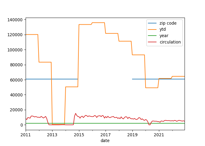
That’s interesting, but by default .plot() will use a
line plot for all numeric variables of the DataFrame. This isn’t exactly
what we want, so let’s tell .plot() what variable to use by
selecting the circulation column.
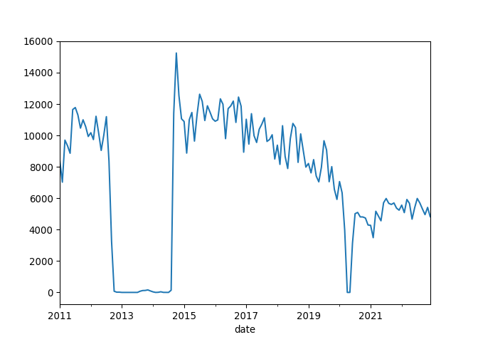
Analyze the Circulation Trends
Examine the line graph depicting library circulation data. You will notice two significant periods where the circulation drops to zero: first in March 2020 and then a two-year zero circulation period starting in 2012. Evaluate the graph and identify any trends, unusual patterns, or notable changes in the data.
The significant drop in circulation in March 2020 is likely due to the COVID-19 pandemic, which caused widespread temporary closures of public spaces, including libraries.
The drop from 2012 through part of 2014 corresponds to the reconstruction period of the Albany Park Branch. The original building at 5150 N. Kimball Avenue was demolished in 2012, and a new, modern building was constructed at the same site. The new Albany Park Branch opened on September 13, 2014, at 3104 W. Foster Avenue in the North Park neighborhood of Chicago. More details about this renovation can be found on the Chicago Public Library webpage: Chicago Public Library - Albany Park.
Use Pandas for More Detailed Charts
What if we want to alter the axis labels and the title of the graph? Pandas’ built-in plotting functions, which are backended by Matplotlib, allow us to customize various aspects of a plot without needing to import Matplotlib directly.
- We can pass parameters to Pandas’
.plot()function to add a plot title, specify a figure size, and change the color of the line. - Additionally, we can directly set the x and y axis labels within the
.plot()function.
PYTHON
albany['circulation'].plot(title='Circulation Count Over Time',
                                figsize=(10, 5),
                                color='blue',
                                xlabel='Date',
                                ylabel='Circulation Count')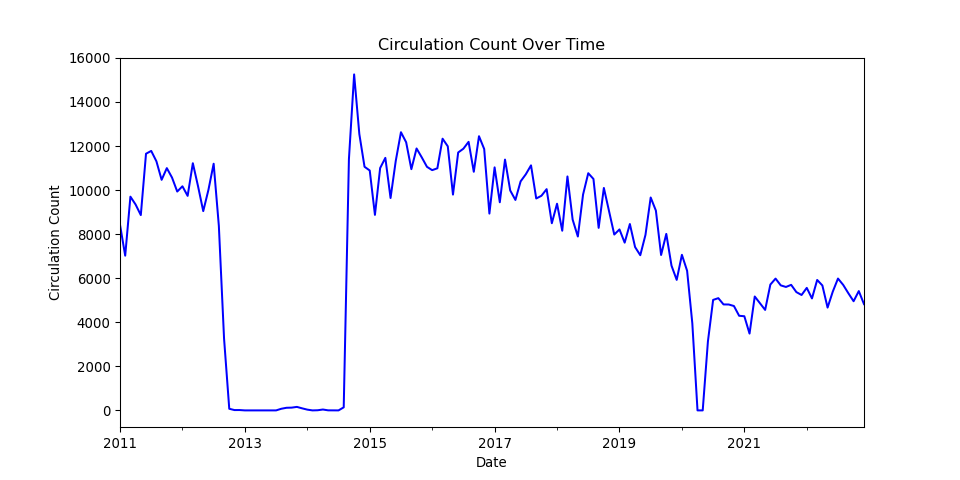
Changing plot types
What if we want to use a different plot type for this graphic? To do
so, we can change the kind parameters in our
.plot() function.
PYTHON
albany['circulation'].plot(kind='area',
                            title='Circulation Count Area Plot at Albany Park', alpha=0.5,
                            xlabel='Date',
                            ylabel='Circulation Count')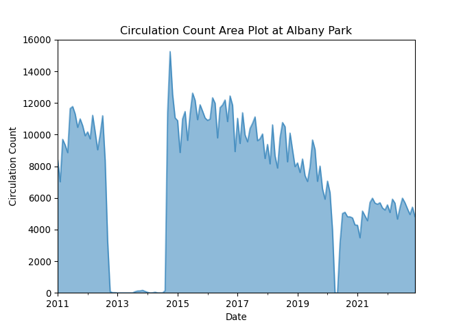
We can also look at our circulation data as a histogram.
PYTHON
albany['circulation'].plot(kind='hist', bins=20,
                            title='Distribution of Circulation Counts at Albany Park',
                            xlabel='Circulation Count')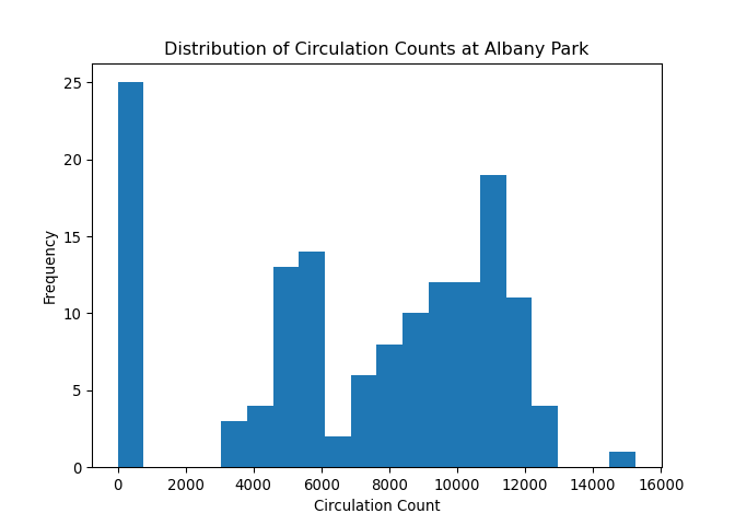
Use Plotly for interactive plots
Let’s switch back to the full DataFrame in df_long and
use another plotting package in Python called Plotly. First let’s
install and then use the package.
PYTHON
# uncomment below to install plotly if the import fails.
# !pip install plotly
import plotly.express as px
Now we can visualize how circulation counts have changed over time for selected branches. This can be especially useful for identifying trends, seasonality, or data anomalies. We willfirst create a subset of our data to look at branches starting with the letter ‘A’. Feel free to select different branches. After subsetting, we will sort our new DataFrame by date and then plot our data by date and circulation count.
PYTHON
# Creating a line plot for a few selected branches to avoid clutter
selected_branches = df_long[df_long['branch'].isin(['Altgeld',
 'Archer Heights',
 'Austin',
 'Austin-Irving',
 'Avalon'])]
selected_branches = selected_branches.sort_values(by='date')
PYTHON
fig = px.line(selected_branches, x=selected_branches.index, y='circulation', color='branch', title='Circulation Over Time for Selected Branches')
fig.show()
Here is a view of the interactive output of the Plotly line chart.
One advantage that Plotly provides over Matplotlib is that it has some interactive features out of the box. Hover your cursor over the lines in the output to find out more granular data about specific branches over time.
Bar plots with Plotly
Let’s use a barplot to compare the distribution of circulation counts among branches. We first need to group our data by branch and sum up the circulation counts. Then we can use the bar plot to show the distribution of total circulation over branches.
PYTHON
# Aggregate circulation by branch
total_circulation_by_branch = df_long.groupby('branch')['circulation'].sum().reset_index()

# Create a bar plot
fig = px.bar(total_circulation_by_branch, x='branch', y='circulation', title='Total Circulation by Branch')
fig.show()
Here is a view of the interactive output of the Plotly bar chart.
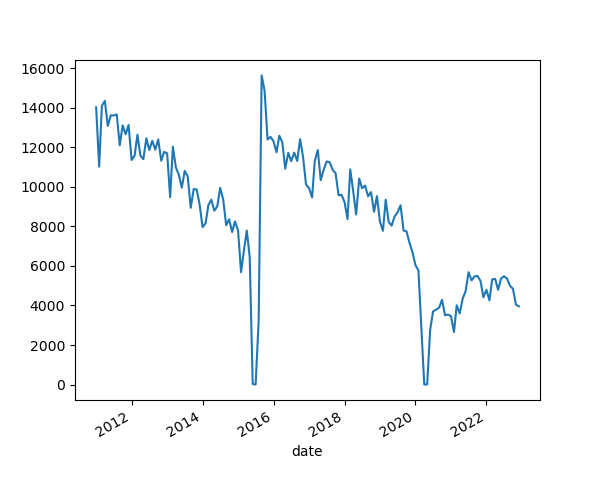
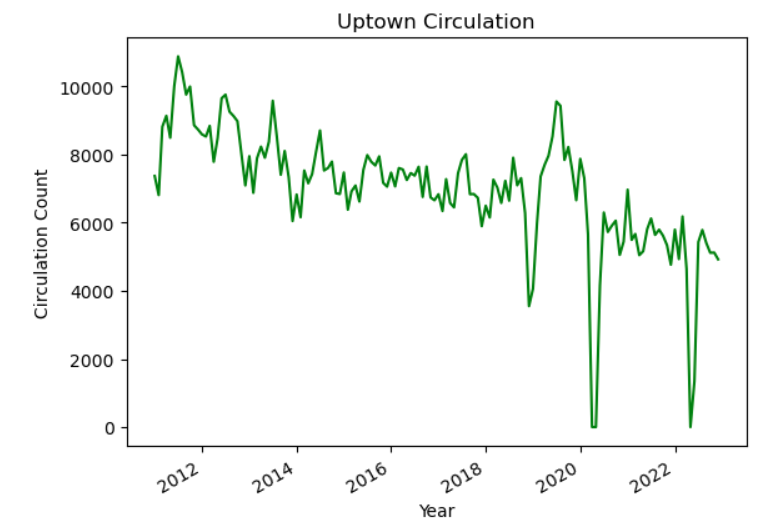
Plot the top five branches
Modify the code below to only plot the five Chicago Public Library branches with the highest circulation.
PYTHON
import plotly.express as px
import pandas as pd
df_long = pd.read_pickle('data/df_long.pkl')
total_circulation_by_branch = df_long.groupby('branch')['circulation'].sum().reset_index()

top_five = total_circulation_by_branch.___________________

# Create a bar plot
fig = px.bar(top_five._______, x='branch', y='circulation', width=600, height=600, title='Total Circulation by Branch')
fig.show()PYTHON
total_circulation_by_branch.sort_values(by='circulation', ascending=False)
df_long = pd.read_pickle('data/df_long.pkl')
total_circulation_by_branch = df_long.groupby('branch')['circulation'].sum().reset_index()

top_five = total_circulation_by_branch.sort_values(by='circulation', ascending=False)

# Create a bar plot
fig = px.bar(top_five.head(), x='branch', y='circulation', width=600, height=600, title='Total Circulation by Branch')
fig.show()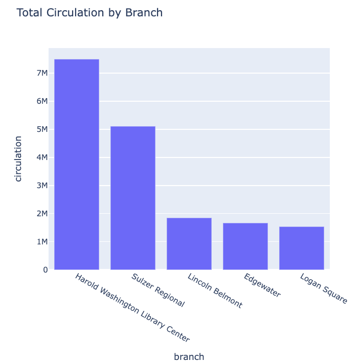
Key Points
- Explored the use of pandas for basic data manipulation, ensuring correct indexing with DatetimeIndex to enable time-series operations like resampling.
- Used pandas’ built-in plot() for initial visualizations and faced issues with overplotting, leading to adjustments like data filtering and resampling to simplify plots.
- Introduced Plotly for advanced interactive visualizations, enhancing user engagement through dynamic plots such as line graphs, area charts, and bar plots with capabilities like dropdown selections.
Content from Wrap-Up
Last updated on 2024-03-23 | Edit this page
Overview
Questions
- What have we learned?
- What else is out there and where do I find it?
- How can I make my programs more readable?
Objectives
- Name and locate scientific Python community sites for further learning.
- Use Python community coding standards (PEP-8).
- Reflect on what you learned.
Python Resources
There are tons of Python resources out there, and Google is generally a good place to start when it comes to troubleshooting Python errors or finding tutorials. A few resources that we recommend:
-
PEP8 is a
style guide for Python that discusses topics such as how you should name
variables, how you should use indentation in your code, how you should
structure your
importstatements, etc. Following PEP8 guidelines makes it easier for other Python developers (and for your future self) to read and understand your code. - The Python 3 documentation covers the core language and the standard library.
- Pandas is the home of the Pandas data library.
- Stack Overflow is a helpful site collecting community questions and answers related to programming challenges. Most of the issues you’re likely to run into as a Python novice have probably been answered there.
Generative AI and Python
Generative AI tools such as ChatGPT, Genesis, and Claude can often generate helpful code templates and suggestions for Python problems. These tools work best:
- when you structure your questions using pseudocode, by breaking down the programming task you hope to accomplish using natural language.
- when you have enough experience in Python that you can troubleshoot errors and read over the code to ensure it’s doing what you think it is. The Python code that ChatGPT suggests can be flawed in small (and sometimes large) ways. You’ll have more success using generative AI for programming help as you gain more experience writing and editing Python.
Reflection
Take a few minutes to think about what you learned during the workshop. Consider the following:
- Are there ways for you to implement Python in your work moving forward?
- Do you have any questions or confusion about how you might implement Python in a particular workflow?
With the time remaining, discuss these topics with your instructors, helpers, and co-learners.