Tidy Data with Pandas

Last updated on 2024-06-14 | Edit this page

Overview

Questions

What are the benefits of transforming data into a tidy format for analysis?
How does the melt() function in pandas facilitate data tidying?
What are some practical challenges when working with real-world datasets in Python, and how can they be addressed?

Objectives

Identify the characteristics of tidy data and explain its benefits, listing the three principles and discussing how it facilitates data analysis during a review session.
Use pandas functions like concat(), melt(), and data filtering to manipulate and clean a complex dataset, successfully combining multiple files into a single DataFrame and reshaping it using melt()

Tidy Data in Pandas

Let’s import the pickle file that contains all of our Chicago public library circulation data in a single DataFrame. We can use the Pandas .read_pickle() method to do so.

PYTHON

import pandas as pd

df = pd.read_pickle('data/all_years.pkl')
df.head()

	branch	address	city	zip code	january	february	march	april	may	june	july	august	september	october	november	december	ytd	year
0	Albany Park	5150 N. Kimball Ave.	Chicago	60625.0	8427	7023	9702	9344	8865	11650	11778	11306	10466	10997	10567	9934	120059	2011
1	Altgeld	13281 S. Corliss Ave.	Chicago	60827.0	1258	708	854	804	816	870	713	480	702	927	787	692	9611	2011
2	Archer Heights	5055 S. Archer Ave.	Chicago	60632.0	8104	6899	9329	9124	7472	8314	8116	9177	9033	9709	8809	7865	101951	2011
3	Austin	5615 W. Race Ave.	Chicago	60644.0	1755	1316	1942	2200	2133	2359	2080	2405	2417	2571	2233	2116	25527	2011
4	Austin-Irving	6100 W. Irving Park Rd.	Chicago	60634.0	12593	11791	14807	14382	11754	14402	14605	15164	14306	15357	14069	12404	165634	2011

PYTHON

df.tail()

	branch	address	city	zip code	january	february	march	april	may	june	july	august	september	october	november	december	ytd	year
958	Chinatown	2100 S. Wentworth Ave.	Chicago	60616.0	4795	4258	5316	5343	4791	5367	5477	5362	4991	4847	4035	3957	58539	2022
959	Brainerd	1350 W. 89th St.	Chicago	60620.0	255	264	370	386	399	421	337	373	361	276	256	201	3899	2022
960	Brighton Park	4314 S. Archer Ave.	Chicago	60632.0	1394	1321	1327	1705	1609	1578	1609	1512	1425	1603	1579	1278	17940	2022
961	South Chicago	9055 S. Houston Ave.	Chicago	60617.0	496	528	739	775	587	804	720	883	681	697	799	615	8324	2022
962	Chicago Bee	3647 S. State St.	Chicago	60609.0	799	543	709	803	707	931	778	770	714	835	718	788	9095	2022

Let’s take a moment to discuss the setup of our DataFrame. It is structured in what is known as a wide format. This format displays an extensive amount of data directly on the screen, with each month’s circulation counts spread across the columns in a pivoted manner. This layout makes it easier to read and manually manipulate the data in a spreadsheet and because of this, is often the default output for periodic reporting systems like integrated library systems.

However, this wide format can pose challenges when working with data analysis tools like Pandas. For instance, if we need to identify all the library branches where circulation exceeded 10,000 in any given month, we would have to individually check each column dedicated to a month, which can be quite cumbersome.

To address this we can reshape our data in a long format. This is sometimes called un-pivoting the data, and in our case the month columns will become a single variable in the dataset.

Tidy Data

Tidy data is a standard way of organizing data values within a dataset, making it easier to work with. Here are the key principles of tidy data: 1. Every column holds a single variable, like “month” or “temperature.” 2. Every row represents a single observation, like circulation counts by branch and month. 3. Every cell contains a single value.

The image below might help orient us to the concept of tidy data.

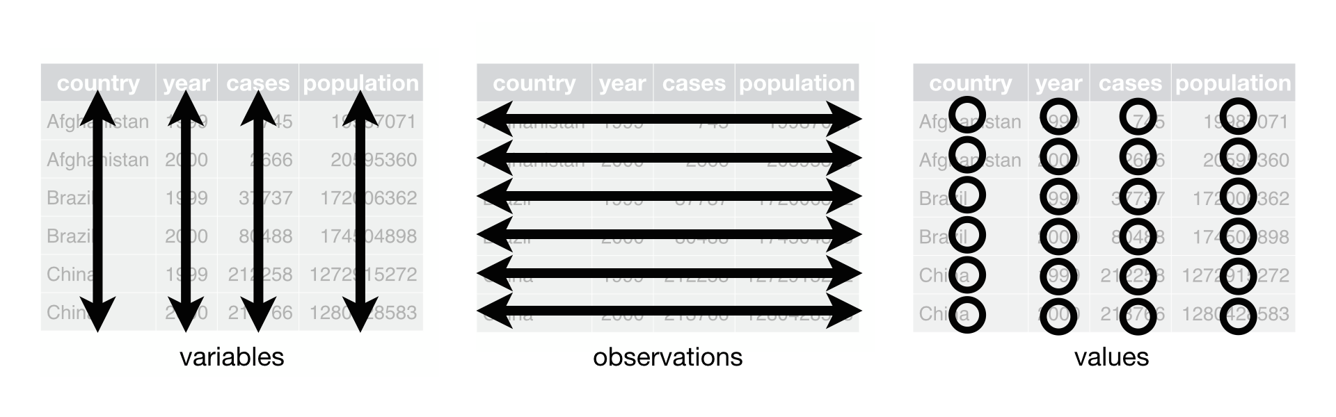
image showing variables in columns, observations in rows, and values in cellssan

R for Data Science 12.1

Benefits of Tidy Data

Transforming our data into a tidy data format provides several advantages: - Python operations, such as visualization, filtering, and statistical analysis libraries, work better with data in a tidy format. - Tidy data makes transforming, summarizing, and visualizing information easier. For instance, comparing monthly trends or calculating annual averages becomes more straightforward. - As datasets grow, tidy data ensures that they remain manageable and analyses remain accurate.

Making Our Data Tidy

A good step towards tidying our data would be to consolidate the separate month columns into a column called month, and the circulation counts into another column called circulation_counts. This simplifies our data and aligns with the principles of tidy data.

To achieve this transformation, we can use a Pandas function called melt(). This function reshapes the data from wide to long format, where each row will represent one month’s circulation data for a branch. Let’s look at the help for melt first.

PYTHON

help(pd.melt)

Now, let’s tidy our data. We’ll create a new dataframe called df_long and use melt to reshape. melt essentially melts down our columns into rows.

PYTHON

df_long = df.melt(id_vars=['branch', 'address', 'city', 'zip code', 'ytd', 'year'],
                    value_vars=['january', 'february', 'march', 'april', 'may', 'june', 
                                'july', 'august', 'september', 'october', 'november', 'december'],
                    var_name='month', value_name='circulation')

In the above code we use id_vars to list the columns we do not want to melt. We then identify the columns we do want to melt into rows in the value_vars parameter. var_name is the variable name for the columns that will be transformed into rows. value_names is the measured variable, circulation in our case. Let’s now look at the new structure of our data.

PYTHON

df_long

	branch	address	city	zip code	ytd	year	month	circulation
0	Albany Park	5150 N. Kimball Ave.	Chicago	60625.0	120059	2011	january	8427
1	Altgeld	13281 S. Corliss Ave.	Chicago	60827.0	9611	2011	january	1258
2	Archer Heights	5055 S. Archer Ave.	Chicago	60632.0	101951	2011	january	8104
3	Austin	5615 W. Race Ave.	Chicago	60644.0	25527	2011	january	1755
4	Austin-Irving	6100 W. Irving Park Rd.	Chicago	60634.0	165634	2011	january	12593
…	…	…	…	…	…	…	…	…
11551	Chinatown	2100 S. Wentworth Ave.	Chicago	60616.0	58539	2022	december	3957
11552	Brainerd	1350 W. 89th St.	Chicago	60620.0	3899	2022	december	201
11553	Brighton Park	4314 S. Archer Ave.	Chicago	60632.0	17940	2022	december	1278
11554	South Chicago	9055 S. Houston Ave.	Chicago	60617.0	8324	2022	december	615
11555	Chicago Bee	3647 S. State St.	Chicago	60609.0	9095	2022	december	788

Ok, let’s look at the unique branches in our long DataFrame:

PYTHON

df_long['branch'].unique()

OUTPUT

array(['Albany Park', 'Altgeld', 'Archer Heights', 'Austin',
       'Austin-Irving', 'Avalon', 'Back of the Yards', 'Beverly',
       'Bezazian', 'Blackstone', 'Brainerd', 'Brighton Park',
       'Bucktown-Wicker Park', 'Budlong Woods', 'Canaryville',
       'Chicago Bee', 'Chicago Lawn', 'Chinatown', 'Clearing', 'Coleman',
       'Daley, Richard J. - Bridgeport', 'Daley, Richard M. - W Humboldt',
       'Douglass', 'Dunning', 'Edgebrook', 'Edgewater', 'Gage Park',
       'Galewood-Mont Clare', 'Garfield Ridge', 'Greater Grand Crossing',
       'Hall', 'Harold Washington Library Center', 'Hegewisch',
       'Humboldt Park', 'Independence', 'Jefferson Park', 'Jeffery Manor',
       'Kelly', 'King', 'Legler Regional', 'Lincoln Belmont',
       'Lincoln Park', 'Little Village', 'Logan Square', 'Lozano',
       'Manning', 'Mayfair', 'McKinley Park', 'Merlo', 'Mount Greenwood',
       'Near North', 'North Austin', 'North Pulaski', 'Northtown',
       'Oriole Park', 'Portage-Cragin', 'Pullman', 'Roden', 'Rogers Park',
       'Roosevelt', 'Scottsdale', 'Sherman Park', 'South Chicago',
       'South Shore', 'Sulzer Regional', 'Thurgood Marshall', 'Toman',
       'Uptown', 'Vodak-East Side', 'Walker', 'Water Works',
       'West Belmont', 'West Chicago Avenue', 'West Englewood',
       'West Lawn', 'West Pullman', 'West Town', 'Whitney M. Young, Jr.',
       'Woodson Regional', 'Wrightwood-Ashburn', 'Little Italy',
       'West Loop'], dtype=object)

Alright! Now that we have the data tidied what can we do with it? Let’s look at which branches circulated over 10,000 items in any given month. We can filter the df_long DataFrame to only show rows that have a number greater than 10,000 in the circulation column.

PYTHON

df_long[df_long['circulation'] > 10000]

	branch	address	city	zip code	ytd	year	month	circulation
4	Austin-Irving	6100 W. Irving Park Rd.	Chicago	60634.0	165634	2011	january	12593
12	Bucktown-Wicker Park	1701 N. Milwaukee Ave.	Chicago	60647.0	173396	2011	january	13113
13	Budlong Woods	5630 N. Lincoln Ave.	Chicago	60659.0	160271	2011	january	12841
17	Chinatown	2353 S. Wentworth Ave.	Chicago	60616.0	158449	2011	january	14027
24	Edgebrook	5331 W. Devon Ave.	Chicago	60646.0	129288	2011	january	10231
…	…	…	…	…	…	…	…	…
11373	Harold Washington Library Center	400 S. State St.	Chicago	60605.0	276878	2020	december	20990
11420	Sulzer Regional	4455 N. Lincoln Ave.	Chicago	60625.0	260163	2021	december	21671
11454	Harold Washington Library Center	400 S. State St.	Chicago	60605.0	271811	2021	december	21046
11532	Harold Washington Library Center	400 S. State St.	Chicago	60605.0	273406	2022	december	20480
11545	Sulzer Regional	4455 N. Lincoln Ave.	Chicago	60625.0	301340	2022	december	21258

1434 rows × 8 columns

We can look at specific columns:

PYTHON

df_long[['branch', 'circulation']]

	branch	circulation
0	Albany Park	8427
1	Altgeld	1258
2	Archer Heights	8104
3	Austin	1755
4	Austin-Irving	12593
…	…	…
11551	Chinatown	3957
11552	Brainerd	201
11553	Brighton Park	1278
11554	South Chicago	615
11555	Chicago Bee	788

11556 rows × 2 columns

We can sort our table using .sort_values() to see the branches with the highest circulation per month:

PYTHON

df_long.sort_values('circulation', ascending=False)

	branch	address	city	zip code	ytd	year	month	circulation
1957	Harold Washington Library Center	400 S. State St.	Chicago	60605.0	966720	2011	march	89122
2920	Harold Washington Library Center	400 S. State St.	Chicago	60605.0	966720	2011	april	88527
2999	Harold Washington Library Center	400 S. State St.	Chicago	60605.0	937649	2012	april	87689
6772	Harold Washington Library Center	400 S. State St.	Chicago	60605.0	966720	2011	august	85193
2036	Harold Washington Library Center	400 S. State St.	Chicago	60605.0	937649	2012	march	84255
…	…	…	…	…	…	…	…	…
3623	Portage-Cragin	5108 W. Belmont Ave.	Chicago	60641.0	36262	2020	april	0
3622	Manning	6 S. Hoyne Ave.	Chicago	60612.0	3325	2020	april	0
3621	Daley, Richard J. - Bridgeport	3400 S. Halsted St.	Chicago	60608.0	37045	2020	april	0
3620	Canaryville	642 W. 43rd St.	Chicago	60609.0	4120	2020	april	0
3577	Merlo	644 W. Belmont Ave.	Chicago	60657.0	14637	2019	april	0

11556 rows × 8 columns

What if we want to tally up the total circulation for each branch over all years and also see the mean circulation?

PYTHON

df_long.groupby('branch')['circulation'].agg(total_circulation='sum', mean_circulation='mean')

	total_circulation	mean_circulation
branch
Albany Park	1024714	7116.069444
Altgeld	68358	474.708333
Archer Heights	803014	5576.486111
Austin	200107	1389.631944
Austin-Irving	1359700	9442.361111
…	…	…
West Pullman	295327	2050.881944
West Town	922876	6408.861111
Whitney M. Young, Jr.	259680	1803.333333
Woodson Regional	823793	5720.784722
Wrightwood-Ashburn	302285	2099.201389

82 rows × 2 columns

df.groupby('branch'): This groups the data by the ‘branch’ column so that all entries in the DataFrame with the same library branch are grouped together. (This is similar to the SQL GROUP BY statement or the group_by function in dplyr in R.)
['circulation']: After grouping the data by branch, this specifies that subsequent operations should be performed on the ‘circulation’ column.
.agg(...): The agg function is used to apply one or more aggregation operations to the grouped data. Inside the agg function:
- total_circulation='sum': This creates a new column named ‘total_circulation’ where each entry is the sum of ‘circulation’ for that branch. It totals up all circulation figures within each branch.
- mean_circulation='mean': This creates a new column named ‘mean_circulation’ where each entry is the average ‘circulation’ for that branch. It calculates the mean circulation figures for each branch.

If we want to group by more than one variable, we can list those column names in the .groupby() function.

PYTHON

df_long.groupby(['branch', 'month'])['circulation'].agg(['sum', 'mean'])

		sum	mean
branch	month
Albany Park	april	79599	6633.250000
	august	91416	7618.000000
	december	77849	6487.416667
	february	76747	6395.583333
	january	85952	7162.666667
…	…	…	…
Wrightwood-Ashburn	march	25817	2151.416667
	may	22049	1837.416667
	november	24124	2010.333333
	october	27345	2278.750000
	september	25692	2141.000000

984 rows × 2 columns

Adding a Date Column

In order to plot this data over time in the data visualization we need to do three things to prepare it. First, we need to combine the year and month columns into its own column. Second, convert the new date column to a datetime objec using the Pandas to_datetime function. Third, we assign the date column as our index for the data. These steps will set up our data for plotting.

PYTHON

df_long['date'] = df_long['year'] + '-' + df_long['month']

This will create a new column in our data frame by adding our year and month together separated by a -. This setup is not sufficient for us to use .to_datetime() to convert the column to something Python and Pandas knows is a date.

PYTHON

df_long['date'] = pd.to_datetime(df_long['date'], format='%Y-%B')

pd.to_datetime() will do the conversion, but we need to tell it how we have our date formatted. In this case we have year and month name spelled out. To find more format codes, see https://docs.python.org/3/library/datetime.html#strftime-and-strptime-behavior.

If we take a look at the date column, we’ll see that datetime automatically adds a day (always 01) in the absence of any specific day input.

PYTHON

df_long['date']

OUTPUT

0       2011-01-01
1       2011-01-01
2       2011-01-01
3       2011-01-01
4       2011-01-01
           ...    
11551   2022-12-01
11552   2022-12-01
11553   2022-12-01
11554   2022-12-01
11555   2022-12-01
Name: date, Length: 11556, dtype: datetime64[ns]

PYTHON

df_long.info()

OUTPUT

<class 'pandas.core.frame.DataFrame'>
RangeIndex: 11556 entries, 0 to 11555
Data columns (total 9 columns):
 #   Column       Non-Null Count  Dtype         
---  ------       --------------  -----         
 0   branch       11556 non-null  object        
 1   address      7716 non-null   object        
 2   city         7716 non-null   object        
 3   zip code     7716 non-null   float64       
 4   ytd          11556 non-null  int64         
 5   year         11556 non-null  object        
 6   month        11556 non-null  object        
 7   circulation  11556 non-null  int64         
 8   date         11556 non-null  datetime64[ns]
dtypes: datetime64[ns](1), float64(1), int64(2), object(5)
memory usage: 812.7+ KB

That worked! Now, we can make the datetime column the index of our DataFrame. In the Pandas episode we looked at Pandas default numerical index, but we can also use .set_index() to declare a specific column as the index of our DataFrame. Using a datetime index will make it easier for us to plot the DataFrame over time. The first parameter of .set_index() is the column name and the inplace=True parameter allows us to modify the DataFrame without assigning it to a new variable.

PYTHON

df_long.set_index('date', inplace=True)

If we look at the data again, we will see our index will be set to date.

Let’s save df_long to use in the next episode.

PYTHON

df.to_pickle('data/df_long.pkl')

Tidy Data Principles

How would you reorganize the following table about research data workshops to follow the three tidy data principles?

Every column holds a single variable.
Every row represents a single observation.
Every cell contains a single value.

Date	Length	Content	Instructor
2023-01-15	30 min	RDM, DMP	CH
2023-02-02	2 hours	Python, RDM	CH, TD
2023-02-03	90 min	Python	SP

You can use each content unit (e.g., RDM, DMP, Python) as an observation, and breakdown the length of time or instructor initials to match the content unit however you like.

Show me the solution

Year	Month	Day	Length (min)	Content	Instructor
2023	01	15	20	RDM	CH
2023	01	15	10	DMP	CH
2023	02	02	100	Python	TD
2023	02	02	20	RDM	CH
2023	02	03	100	Python	SP

Subsetting df_long

Using df_long, create a new DataFrame, `low_circ’, that only includes branches with circulation numbers lower than 500 per month. When you create a subset DataFrame, show the following columns: branch, circulation, month, and year. Next, eliminate the rows when the circulation is equal to 0.

PYTHON

low_circ = df_long[_________[_________] __ 500]
low_circ = _________[_________[_________] != __]
low_circ.sort_values(by='circulation', ascending=False)

Show me the solution

PYTHON

low_circ = df_long[df_long['circulation'] < 500]
low_circ = low_circ[low_circ['circulation'] != 0]
low_circ.sort_values(by='circulation', ascending=False)

Group and aggregate for circulation by year

How would you create a subset of df_long that sums up the circulation by year across all branches? In other words you want a view of the DataFrame that includes one row for each year, and columns for ‘year’ and ‘sum’, the latter of which shows the sum of circulation for all branches in each year.

Show me the solution

PYTHON

df_long.groupby(['year'])['circulation'].agg(['sum'])

year	sum
2011	7774198
2012	7598080
2013	6894958
2014	6406512
2015	5953920
2016	5696456
2017	5305624
2018	4989239
2019	4785108
2020	2726156
2021	3184327
2022	3342472

Key Points

In tidy data each variable forms a column, each observation forms a row, and each type of observational unit forms a table.
Using pandas for data manipulation to reshape data is fundamental for preparing data for analysis.